traffic assignment code in matlab

An official website of the United States government

The .gov means it’s official. Federal government websites often end in .gov or .mil. Before sharing sensitive information, make sure you’re on a federal government site.

The site is secure. The https:// ensures that you are connecting to the official website and that any information you provide is encrypted and transmitted securely.

• Publications
• Account settings

Preview improvements coming to the PMC website in October 2024. Learn More or Try it out now .

• Advanced Search
• Journal List

Matlab algorithms for traffic light assignment using fuzzy graph, fuzzy chromatic number, and fuzzy inference system

Isnaini rosyida.

a Universitas Negeri Semarang, Indonesia

  Nurhaida

b Universitas Papua, Indonesia

Alfa Narendra

  widodo.

c Universitas Gadjah Mada, Indonesia

We propose algorithms in Matlab that combine fuzzy graph, fuzzy chromatic number (FCN), and fuzzy inference system (FIS) to create traffic light assignment based on traffic flow, conflict, and queue length in an intersection. We evaluate the algorithms through two case studies each on a signalized intersection at Semarang City (Indonesia) and compare the result to the existing systems. The case studies show that the algorithm based on fuzzy graph-FCN-FIS could reduce traffic light cycle time on the intersections.

We provide three results as follows:

• • A pseudocode to construct fuzzy graph of traffic data in an intersection.
• • Algorithm 1 is to Determine fuzzy graph model of a traffic light data and phase scheduling using FCN function which is presented using Matlab programming language.
• • Algorithm 2 is to Determine duration of green lights of each phase using Mamdani-FIS codes in Matlab.

Graphical abstract

Specifications table

Method details

Throughout this paper, we use some terms in traffic light problems. A phase on an intersection is a portion of a signal cycle when the green lights are assigned to a certain combination of traffic movements. Traffic flow is the study of the movement of individual drivers and conveyances among two locations and the interactions between them. Meanwhile, a volume is defined as a number of traffic elements flowing an area on a road per unit of time (vehicles/hour or passenger car unit/hour) [1] . One of the most important problems that is needed to be solved is traffic congestion. In Indonesia, generally, a fixed phase and fixed time period of green lights on each phase are common applied on an intersection. In this case, whether there are or none vehicles passing through the intersection, the green light is still on until the time elapses. This condition will lead to accumulating queue on a lane with a high traffic volume, particularly at peak hour. One of the alternative options is to create a traffic assignment where the phase scheduling applied considers traffic flow, conflict, and queue. We call this state as a fuzzy phase scheduling.

In general, we model traffic flow on an intersection by using classical graph G ( V , E ) where V a vertex set and E an edge set, represent a set of traffic flows and a set of conflicting traffic flows, respectively. Two vertices that are connected by an edge mean that the flows are in conflict and should be assigned in different phases. In modeling traffic flow using graph vertex coloring, a color represents a phase on an intersection. A minimum number of colors used in the vertex coloring of G , called as chromatic number, represents a minimum number of phases required on the intersection. Given the load of traffic volumes on conflicting flows, it is interesting to figure out safety level on these flows. Moreover, a conflict between two traffic flows cannot be predicted exactly because it highly depends on their traffic volumes which vary and fluctuate in time. In other words, magnitudes of the conflict exhibit fuzzy phenomena. Hence, we need an alternative graph that accommodates indeterminate phenomena on conflicting traffic flows to model traffic light assignments. Therefore, we proceed to model traffic flows in an intersection in a fuzzy graph where, on each edge, we assign a degree of membership that represents a degree of conflict between two vertices. Next, by using fuzzy chromatic number (FCN) of the graph we produce the number of phases, their respective degree of safety and their phase scheduling. We choose, heuristically a set of phase schedulings to be implemented in an intersection. By setting queue length of flows in a phase scheduling as the inputs and duration of green light as the output of a Mamdami-FIS, we are able to get the desire traffic assignment which the green light setting considering the queue length of the respective flows. This assignment, as can be seen later, has shorter cycletime compared to fixed green duration setting. Further, we use term “traffic flows” in place of “traffic movements” and vice versa, both to describe vertices.

In one hand, several researchers studied traffic light problems using fuzzy graph in [2] , [3] , [4] , [5] – 6] , However, these works studied only on fixed phases and none of these works gave fuzzy phase scheduling and computation of their proposed method. In other hand, many researchers applied only fuzzy logic in traffic light problems. The application of fuzzy logic i.e., Fuzzy Inference System (FIS), in traffic control was first initiated by Pappis and Mamdani [7] . Later, many researchers discussed this problem, such as in [8] , [9] , [10] , [11] , [12] , [13] , [14] – 15] . In contrast to other research of traffic light based on fuzzy graph or FIS, this research focuses on constructing fuzzy phase scheduling that links fuzzy graph, FCN and FIS.

Different traffic flows on different conditions ideally require different phase scheduling. Hence, it can be said that setting an optimal phase is a fuzzy phenomenon. In this research, we propose a phase scheduling that considers traffic intensities using fuzzy graph and FCN. Firstly, we construct an algorithm in Matlab to model a traffic light system using fuzzy graph. Secondly, we determine the phase scheduling using FCN algorithm and calculate duration of green lights using Mamdani-FIS function in Matlab. The concept and algorithm of FCN were given in the main article [16 , 17] . Basic terminologies used in the algorithm are presented in the appendix.

The algorithm is divided into two parts as follows:

• 1. Determining fuzzy graph model of a traffic light system and phase scheduling using FCN function.
• 2. Determining duration of green lights of the phases in part (1) using Mamdani-FIS codes in Matlab.

Determining fuzzy graph and phase scheduling

We constrcut a pseudocode to represent traffic data in an intersection into a fuzzy graph as shown in Table 1 .

Pseudocode to construct fuzzy graph of traffic data in an intersection.

Data of traffic are first inputed into a mat file. The following scripts are used.

As shown on the above script, we use an intersection with 4 approaches, namely: W=west, N=north, E=east, and S=south. If users want to applied this program in an intersection with more than 4 approaches, than they can modify these commands. There are 4 inputs. Flows is a set of traffic flows which are represented as vertices in the fuzzy graph. Flow `WN'states that there is a traffic movement from West to North. Users should identify which traffic flows represents the intersection and they can modify this step based on traffic assignments in the intersection. Volumes is a set of the number of vehicles for all traffic flows. The third input is Conflicts. It is a set of conflicting traffic flows. They are represented as edges in the fuzzy graph. For example, let traffic flow `WN’ and SN' are in conflict. Then, there is an edge `WN SN' in the edge set. Lastly, we input Queue, a set of queue length of the flows, Flows. This input, will be used later in the next part. The users can modify this step according to conflicting traffic flows that they are observed in the intersection. Step 1 in the script is the first 3 steps on the pseudocode. The following command on Matlab command window shows the load of mat.file ‘case1.mat’ that we input on the above algorithm.

Further, we create the following algorithm which are based on the above pseudocode and FCN in [17] . We call this algorithm as Algorithm 1 for ease of referencing in this article.

Explanation of Algorithm 1 is as follows:

• In step 1. We load traffic data called case1.
• In step 2, fuzzy graph construction is done. We calculate crisp volume of conflicting movements or crisp weight of edges in step 2.1. In step 2.2 and step 2.3, we determine intervals and fuzzy sets of traffic volumes, i.e., {(low,μ low ), (medium,μ medium ), (high,μ high )} where μ is the membership function and we display the membership functions of the fuzzy sets, respectively. We fuzzify the edge crisp weights in step 2.4 to get the fuzzy edge set, E ˜ = ( E , μ E ) . Plot of the fuzzy graph is given in step 2.5. The script on this step describes step 4 up to the last step in the pseudocode.

Determining the phase scheduling is done in step 3. We use a call function namely FCNwithpartition which is on the appendix B. This function is a slighty modified form of its original flowchart in [17] . Input for this function is a fuzzy edge set, while outputs are k,Lk and P. The output k is chromatic number. In graph traffic modeling, it represents the number of phases. Lk is the degree of safety of its respective value k. Setting both side by side, we get (k,Lk) is the fuzzy chromatic number. The output P is the associated phase scheduling to the number of phases k. Also, known as k-phase scheduling. Saving the phase scheduling in a mat file to be processed further as input for the second part of the modeling is done in the last step, step 4.

The result of Algorithm 1 is a mat file called, in this example, 'case1_FuzzyPhases.mat'. The following scripts on Matlab Command Window show the content of the file. There are three commands on the window. The first command is to load  the mat file. The file contains one structure namely Patterns. The second command is to check the contents of Patterns. There are four substructures on Patterns. The last command, Patterns. FuzzyChromaticNumber displays FCN, i.e., the number of minimum phases, k and its respective degree of safety, Lk.

The next step is to determine phases which are eligible for fuzzy phase scheduling. Given that FCN shows safety level of the number of phases applied on the traffic network, to be eligible, we can determine the k-phase based on the degree. We omit the case of k  = 1, i.e. 1-phase scheduling, as definitely not safe (see the above scripts). Meanwhile, arrangement with 3 to 8 phases have 1 safety level. However, as the number of phases applied on an intersection affects the length of cycle time, of all the number of phases which has 1 safety degree we choose the smallest number. In this example, we choose k  = 3. By that setting we work only on k  = 2 and k  = 3 phases. The last 2 substructures on Patterns, i.e., for_3phase and for_2phase, show all possible patterns of their k-phase.

As mentioned previously, chromatic number (k) represents the number of phases in a traffic assignment. A term k-phase scheduling means we assign k phases for traffic assignment on an intersection. Fuzzy chromatic number (k,Lk) gives a degree of applying k-phase scheduling in a traffic assignment. As shown on FCN on the above scripts, 1-phase scheduling comes with the lowest degree (0.0041), as it is obviously not safe if traffic elements are allowed to flow (from all directions) all at once. Assignments within 2 phases comes with higher degree which is 0.5723. Whereas, assignments within 3 or more phases has 1 degree of safety. However, the more the number of phases the lengthier the traffic cycle time. There is inevitably a trade-off between safety level and cycle time length. Therefore, we are looking for a phase scheduling which is safe at a reasonable cycle time.

Determining duration of green light

Having constructing traffic phases, we would like to determine duration of the traffic lights which considers queue length of flows on the phases. This is done by Mamdami-FIS codes. The highligth of the system is as follows:

• 1. The input parameter is flowing queue length in each phase and is labelled as Short, Medium, Long. The formula used to determine the queue length in each traffic flow is presented in Eqn 1 : Ql = ∑ i = 1 3 ( L i × Q i ) c × width (1)

where Ql is the queue length (meter), L i is the area of each vehicle-i (m 2 ), Q i is the number of vehicles per hour, c is the number of cycles of green light per hour, width is the wide of the approach (meter), and i is the type of vehicle (i=1 for MC(Motor Cycle), i=2 for LV(Light Vehicle), and i=3 for HV(Heavy Vehicle)).

• 2. The output parameter is green light-duration in each phase (Short, Medium, Long). According to standard cycle time for the 3-phase or 4-phase scheduling [1] , we use the maximum length of interval for the output is 100 s. The fuzzy sets of input and output parameters have triangular membership functions.
• 3. The fuzzy rules are defined based on the number of phases used and maximum traffic flows in a phase.
• 4. The defuzzification method is centroid.

The following matlab algorithm which we call Algorithm 2 is mainly composed of Mamdani-FIS in codes.

Algorithm 2 consists of three main steps. The first step is loading data. We need to input Queue which is in file case1.mat. The queue length of the movements is calculated using the formula in [1] . We load fuzzy phases obtained in the previous algorithm that is in variable Patterns.allphases in case2_FuzzyPhases mat file. As our Mamdami input is queue length of flows, we need to fuzzify the queue length into fuzzy sets, i.e., short, medium and long where each has triangular membership function. Hence, we need to load the range inRange and parameters of each membership function inMFparams.

Step 2 is the Mamdami-FIS system written in coding. The number of inputs of the FIS is set to be not more than 4, e.g., Queue-length1, Queue-length2, Queue-length3, and Queue-length4. The label Queue-length1 means the queue length in the first flow and so on. Given any k-phase scheduling, Algorithm 2 will work only if maximum number of flows/movements on the phase scheduling is 2,3 or 4. We limit the algorithm due to the empirical fact that applying a phase with more than 4 flows/movements results in a lengthier cycletime.

There is only one output of our FIS that is duration of green light. The fuzzy output may have three fuzzy numbers ,e.g. {'short';'medium';'long'}. We set maximum duration of green light for a phase is 100 s [1] and set fixed parameters for triangular membership function as [0 0 35; 30 50 70; 60 100 100], respectively. We call our Mamdami-FIS as ‘fuzzy-traffic’. Three plots in Fig. 1 show available systems of the FIS stucture, i.e., the input, output and evaluation. As can be seen, we set 9, 27 and 15 rules for 2, 3 and 4 inputs, respectively. One can see that we use a call function getmyrule() as in command rule = getmyrule(numOfinLabels)in Step 2 Algorithm 2. We give this function in Appendix C .

`Fuzzy-traffic'. A Mamdami FIS for k-fuzzy phase scheduling.

In step 3, we save all the outputs. By inputting fuzzy phases obtained previously, ‘fuzzy-traffic’ system gives one phase scheduling that is a scheduling for 3 phases. The result is in a mat file namely 'case1_3-FuzzyPhaseScheduling.mat' (see the scripts below). There are 5 options of phase patterns to arrange the traffic using 3 phases. We can see the results interactively in Variable Window as well.

Experimental results

Location 1 (kaligarang intersection, semarang city, central java, indonesia).

Let us consider a case study on an intersection in Semarang City, Central Java, Indonesia, particularly in “Kaligarang” intersection [18] . Fig. 2 shows the sketch and image of the intersection. Data of traffic volumes on all movements are gathered by using video camera during week days (Monday, Tuesday, and Wednesday) on August 6–8, 2018. The data was taken four hours each day e.g., during two peak hours in the morning (06.00–08.00 a.m.) and two peak hours at afternoon (16.00–18.00 p.m.). Data of this example have been shown to illustrate the building of our algorithms (1 and 2).

Sketch (left) and image (right) of traffic light system in Kaligarang intersection (Location 1) [18] .

We call this example as case 1. There are four variables to model the intersection into a fuzzy graph. These are traffic flows, traffic volumes, flow queue length and conflicting flows. The first three variables are shown in Table 2 and the fourth variable is on the 2nd or 3rd column of Table 3 . Traffic flows and their volumes are used in Algorithm 1. Whereas, queue length is used in Algorithm 2. As said in introduction, in graph modeling, traffic flows and conflicting flows are modeled as vertex ( V ) and edge ( E ) sets, respectively. In our model, we use fuzzy edge set E ˜ = ( E , W ) that is we assign a degree to each edge in E . In doing so, we define membership functions for traffic volumes, i.e., fuzzy sets of traffic volumes. We then construct fuzzy graph of the traffic data, G ˜ = ( V , E ˜ ) . Plots of the membership functions and fuzzy graph are shown in Fig. 3 . Both plots are the outputs of step 2 in Algorithm 1.

Traffic flows, volumes and queue length at Location 1 during peak time (morning).

Conflicting traffic flows (edge set), volumes, and their membership degrees

Membership functions of fuzzy edge set in Table 3 (left) and representation of traffic in Fig. 2 into a fuzzy graph (right).

As stated previously, output of the first algorithm is fuzzy phases of an intersection. The phases are defined as “fuzzy” because based on FCN definition, a level of safety is assigned to each number of phases. Table 6 shows FCN of traffic network of case 1. The table is interactively screenshootted and cropped from Matlab Variable Window. The number k in Table 4 represents the amount of phases to arrange traffic flows, while Lk represents a possibility to apply the k -phase. According to the table, traffic assignment with 3 number of phases on Location 1 has one degree of safety. Therefore, we can apply k  = 3 phases during peak time, i.e., between 06.30–09.00 a.m. or between 16.00–18.00 p.m. All possible k-phase scheduling with k  = 2 and 3 can be seen on Patterns structure (on the Variable Window) as on the screenshots in Table 5 .

Number of phases (k) and the associated degree (Lk) in case 1.

All possible patterns of k-phase for k  = 2 (top) and k  = 3 (bottom) in case 1.

The 1st option of scheduling with 2-phase in Table 5 .

Table 5 is comprised of two sub tables. The top and bottom sub tables show options of phases of two and three- phase scheduling, respectively. There are 2 options for 2-phase scheduling whereas 5 alternatives are available for 3-phase scheduling. Table 6 and Table 7 show the first option in 2 and 3-phase scheduling, respectively. As can be seen on these two arrangements, maximum number of movements in 2 phases is 6, whereas maximum number of movements for 3 phases is 4. Later, in the second algorithm which constitutes Mamdami-FIS, we limit the algorithm to proceed only phase schedulings where maximum number of the flows are 2, 3, or 4. This is due to empirical facts that more number of movements/flows in a phase increases the cycle time of the assignment.

The 1st option of scheduling with 3-phases in Table 5 .

The next step is to determine green light duration on each phase. The inputs are fuzzy phases shown in Table 5 . that is k  = 3 and k  = 2 fuzzy phases. The system “fuzzy-traffic” reads these inputs and automatically produces the k-phase scheduling according to the rules created. The name of the output mat file is dynamicaly coding, i.e., the algorithm sets the name based on the number of phases of the phase scheduling that is executed online in the system. Hence, the results may be more than one mat file.

For case 1, we obtain a mat file output named ‘result1_3-FuzzyPhaseScheduling.mat’. It means that the available phase scheduling is only one for this case which is the fuzzy scheduling with 3 phases. There are 5 options of phase patterns suggested in the file. Subtables in Table 8 display duration of traffic lights (in seconds) of their respective scheduling with 3 phases shown on screenshots of Matlab Variable Window. One can see that a phase which has on average higher queue will be assigned longer green time.

Duration of green, red, and yellow lights of 3-phase scheduling in Location 1 (Morning).

The 5th pattern of phases in the phase scheduling (on the bottom on Table 8 ) has similar pattern to three phase scheduling in the existing system shown in Table 9 . We can see that the proposed fuzzy phase scheduling reduces cycle time of the traffic light system, i.e. cycle time of the proposed phase scheduling, has lower length. Therefore, the proposed method offers a valuable alternative traffic assignment with 3 phases on the intersection.

Duration of green, red, and yellow lights of the existing system in Location 1 (Morning).

Location 2 (Lamper Gadjah intersection, Semarang City, Central Java, Indonesia)

Let us consider the second case study at Lamper Gadjah intersection in Semarang City, Central Java, Indonesia. Fig. 4 . displays the schema and image of Lamper intersection. Data of traffic volumes acquired from video camera during week days (Monday-Friday) on August 2018 [25] . The data was taken on one hour each day e.g., during peak hour in the afternoon (16.00–17.00 p.m.). Data of this example is inputed and saved as ‘case2.mat’. In Table 10 and Table 11 , we present traffic flows, volumes, queue length and conflicting flows at peak hour and it membership degrees. Further, Step 2 in Algorithm 1 displays plots of membership functions for the edge set and plot of the fuzzy graph ( Fig. 5 ).

Schema (left) and image (right) of traffic light system in Lamper intersection (Location 2) [19] .

Traffic flows, volumes, and queue length at location 2 during peak time (afternoon).

Conflicting traffic flows (edges), volumes and their membership degrees for case 2.

Membership functions of fuzzy edge set (left) and representation of traffic light in Fig. 4 into a fuzzy graph (right).

Number of phases and its level of safety, the result of FCN function, for case 2 is shown in Table 12 . It is shown that assignments with at least 4 phases have degree of safety 1, whereas assignments with less number of phases, i.e., k  = 3, 2 and k  = 1 have very low degree of safety. The function also give all possible phase patterns for k  = 2,3, and 4 as displayed in Table 13 .

Number of phases (k) and the associated degree (Lk) for case 2.

All possible k-phase patterns for k  = 2, 3, and 4 for case 2.

All possible phases in Table 13 are then inputed into the second algorithm. However, we need to put in mind that only scheduling with 4 phases that has 1 degree of safety, the other two have very low degrees of safety (see Table 12 ). We input the range of input variable as [0 140] and intervals of membership functions of input variabels as in inMFparams=[0 0 50; 45 70 95; 90 140 140] (see Algorithm 2).

Two mat files pop up as the result of algorithm 2 suggesting that there are 2 types of phase scheduling. There is only one option in arranging the traffic light in 3 phases ( Table 14 ), whereas, three options are for scheduling with 4 phases ( Table 15 ). In order to validate the result we collect duration of green lights in the existing system (Location 2) which is presented in Table 16 . The system is an intersection where 4-phase scheduling is implemented. The scheduling is equal to the second phase pattern in the fuzzy scheduling with 4 phases (shown on the 2nd subtable from bottom on Table 15 ). We may argue that the fuzzy phase scheduling proposed is superior in reducing the average time a driver spends his/her time on the intersection as the cycle time has shorter length than the cycle time applied in the existing system (in Table 16 ).

Duration of green, red, and yellow lights of 3-phase scheduling in Location 2 (afternoon).

Duration of green, red, and yellow lights of 4-phase scheduling in Location 2 (afternoon).

Duration of green, red, and yellow lights in the existing system (Location 2).

Conclusions

We proposed algorithms to determine the number of phases and the fuzzy phase scheduling for a traffic light system based on fuzzy graph and fuzzy chromatic number. Further, we determine duration of green lights in each phase by applying Mamdani-FIS. We evaluate the algorithms through two case studies. The results show that the combination of the algorithms and the Mamdani-FIS gives some options of phase scheduling with different cycle times. The phase scheduling proposed in this research increases performances of intersections under study in that the cycle times of the proposed scheduling are shorter than that of the existing systems. In our future research, we will improve the performance of the algorithms and implement it on various types of intersections.

Acknowledgments

The Authors appreciate the reviewers for their valuable comments to improve the paper. This paper has supported by the research grant from DIPA UNNES under contract number 207.234/UN37/PPK.3.1/2020.

Declaration of Competing Interest

The authors declare that they have no known competing financial interests or personal relationships that could have appeared to influence the work reported in this paper.

In this part, we discuss basic theories used in the algorithms, such as terminologies in traffic light systems ( [1 , 20 , 21] ), fuzzy graph, and fuzzy chromatic number (FCN) ( [16 , 17] ).

Basic terminologies in traffic light systems

Some terminologies in used in this article are as follows:

• 1. an approach is an area for entering vehicles in a traffic facility;
• 2. a traffic conflict , is "an observable event which would end in an accident unless one of the involved parties slows down, changes lanes, or accelerates to avoid collision" [1] . Traffic conflicts are defined by their time-to-collision, post-encroachment-time, and angle of conflict parameters as well as the vehicles' position in time and space.” [24]
• 3. Light Vehicle (LV) is an index for vehicle on four wheels (including passenger cars, oplets, micro buses, pick-ups and micro trucks);
• 4. Heavy Vehicles (HV) is an index for vehicle with two or three wheels (including buses and truck combinations);
• 5. Motor Cycles (MC) is an index of motor vehicle with two or three wheels (including motor cycles and 3-wheeled vehicles);
• 6. Passenger car unit (pcu) is a conversion factor for different vehicle types with regard to their impact on capacity as compared to a passenger car (i.e. for passenger cars and other light vehicles, pcu = 1.0).

Fuzzy graph and fuzzy chromatic number (FCN)

After a concept of fuzzy set was introduced by Zadeh in 1965 [22] , the concept of a fuzzy graph that consists of a crisp vertex set and a fuzzy edge set was initiated by Kaufmann in 1973 [23] . A fuzzy set A ˜ on X is a set { ( a , μ ( a ) ) | a ∈ X } with a membership function μ : X ↦ [ 0 , 1 ] . Further, the classical sets are named as crisp sets.

Given V which is non-empty set and E ⊆ V × V . A fuzzy graph G ˜ = ( V , E ˜ ) consists of a vertex set V and E ˜ which is a fuzzy edge set with μ : V × V ↦ [ 0 , 1 ] as its membership function. Thereafter, the graph G = ( V , E ) is named as a crisp graph. In crisp graphs, a set A is called an independent vertex set if each pair of vertices in A is independent (not adjacent). The concept is generalized into fuzzy graph as follows. Given δ ∈ [ 0 , 1 ] , a fuzzy independent vertex set (FIVS) of G ˜ = ( V , E ˜ ) is a set I ⊆ V which satisfies the condition μ ( x y ) ≤ δ or each pair x , y ∈ I . The FIVS I can be denoted as I δ . Moreover, a k -coloring of G ˜ could be defined through a partition of V into k - FIVS { I 1 δ , I 2 δ , … , I k δ } such that I i δ ∩ I j δ = ∅ for all i ≠ j and I 1 δ ∪ I 2 δ ∪ … ∪ I k δ = V . The minimum k in the k -coloring of G ˜ is named δ -chromatic number of G ˜ , symbolized by χ δ ( G ˜ ) [24] .

Meanwhile, the concept of FCN is as follows. Given a fuzzy graph G ˜ = ( V , E ˜ ) with n vertices. A FCN of G ˜ , symbolized by χ ˜ ( G ˜ ) , is a fuzzy set χ ˜ ( G ˜ ) = { ( k , L χ ˜ ( k ) ) | k = 1 , 2 , … , n } , where L χ ˜ ( k ) = max { 1 − δ | χ δ ( G ˜ ) = k } is a membership degree of k in the FCN [17] .

The Original Frank-Wolfe Algorithm in Octave (MATLAB)

Erik jensen.

I recently took a course in network optimization where we learned a variety of ways to solve the static traffic assignment problem (TAP). For one of our problem sets, we had to use the Frank-Wolfe algorithm in order to define the user equilibrium (UE) in a standard TAP. So why is this interesting? Well, if you like transportation policy it probably is not, although its use in network optimization has influenced transportation system design for many years now. Most software packages have improved upon the original Frank-Wolfe algorithm.

Before I start, if anybody is struggling to understand the concepts I talk about, I highly recommend Sheffi's textbook which is available for free online (legally!). While the book is a little dated nowadays, it is very straightforward (for a book about the static TAP) and the concepts lay the groundwork for understanding modern-day research into traffic assignment.

Note: Equations require javascript, since they're created with Mathjax .

Background and Main Concepts

Thankfully this is not an academic paper, which means Wikipedia is a perfectly acceptable source for information. Moving on to the basic problem statement, if \(f(x)\) is differential convex real function and \(D\) is a compact convex set, then:

$$\min\ f(x),$$ $$\mathrm{s.t.}\ x\in D.$$

Convexity is incredibly important to many optimization techniques. While the Wikipedia article I linked above is far more rigorous in its definition, it's easy to think about this convexity requirement in two dimensions. Consider the decaying sine wave \(y(t)=e^{-t}\cdot\cos(2\pi t)\). A figure of this function is below.

The minimum point of this function in this range is about -0.6 from the graph. However, imagine your starting point is at 1.2. Moving along the descent direction would get you to the minimum point at about 1.5, which corresponds to a y-value of about -0.21. Without convexity, it is easily possible to end up in a local minimum instead of a global one. Moving on, the biggest advantage of this algorithm is that you only have to solve a small linear sub-problem instead of a full projection step. Essentially, for certain types of problems, Frank-Wolfe is much faster to solve. However, a crucial step in the algorithm is solving the shortest path problem. This algorithm needs to solve this problem hundreds (or thousands) of times, so it needs to be fairly efficient. But how do you actually find the shortest path anyway?

Bellman-Ford-Moore Shortest Path Code

You start by giving your origin a 'potential' (the time it takes to get to that node) of 0, and every other node a potential of some large number (MATLAB supports infinity, so I used that). Please note this is not vectorized code, so you probably don't want to use it when working on any networks with more than 4 or 5 nodes. Our professor gave us his code that was vectorized, but I have not obtained his permission to republish it here, so you are stuck with my inefficient version. MATLAB doesn't have any queue data structure (my friend who works there laughed at me when I asked, MATLAB isn't for this kind of thing), so I used CQueue from the MATLAB Workshop . CQueue is slightly faster (according to random internet forum posters...) than importing Java's queuing structure but I don't have Java installed so that wasn't an option anyway. Once again though, vectorized code will be much faster.

Frank-Wolfe Algorithm with Relative Gap Code

Once again, I didn't really bother to vectorize this code. This isn't nearly as big a problem as with the shortest path code though, as the number of iterations for the networks we had to deal with was always less than 250. For a long time, I used the absolute gap instead of the relative gap, and for the larger networks we had to do (400+ nodes), the algorithm wouldn't converge even at 10,000 iterations. For the same problem, it only took 226 iterations to converge. Also, bfsmp.m is my professor's shortest path code, so you would need to change that line if you want to experiment with my code.

So is this useful?

In short, it used to be. Most modelling software nowadays uses more advanced algorithms than the original Frank-Wolfe Algorithm. More importantly though, they do not implement their code in MATLAB/Octave, which is far slower than almost any compiled language. Despite advancements in recent years, the Frank-Wolfe algorithm is still a great introduction to the static traffic assignment problem. While my code is certainly not efficient, hopefully it can still be informative to anyone who is struggling to figure it out.

Sign up for more like this.

Data-Driven Traffic Assignment: A Novel Approach for Learning Traffic Flow Patterns Using Graph Convolutional Neural Network

• Published: 24 July 2023
• Volume 5 , article number  11 , ( 2023 )

Cite this article

• Rezaur Rahman 1 &
• Samiul Hasan 1  

512 Accesses

3 Citations

Explore all metrics

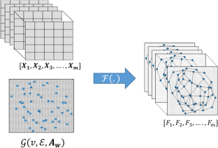
We present a novel data-driven approach of learning traffic flow patterns of a transportation network given that many instances of origin to destination (OD) travel demand and link flows of the network are available. Instead of estimating traffic flow patterns assuming certain user behavior (e.g., user equilibrium or system optimal), here we explore the idea of learning those flow patterns directly from the data. To implement this idea, we have formulated the traditional traffic assignment problem (from the field of transportation science) as a data-driven learning problem and developed a neural network-based framework known as Graph Convolutional Neural Network (GCNN) to solve it. The proposed framework represents the transportation network and OD demand in an efficient way and utilizes the diffusion process of multiple OD demands from nodes to links. We validate the solutions of the model against analytical solutions generated from running static user equilibrium-based traffic assignments over Sioux Falls and East Massachusetts networks. The validation results show that the implemented GCNN model can learn the flow patterns very well with less than 2% mean absolute difference between the actual and estimated link flows for both networks under varying congested conditions. When the training of the model is complete, it can instantly determine the traffic flows of a large-scale network. Hence, this approach can overcome the challenges of deploying traffic assignment models over large-scale networks and open new directions of research in data-driven network modeling.

This is a preview of subscription content, log in via an institution to check access.

Access this article

Price includes VAT (Russian Federation)

Instant access to the full article PDF.

Rent this article via DeepDyve

Institutional subscriptions

Similar content being viewed by others

Modeling Urban Traffic Data Through Graph-Based Neural Networks

Predicting Taxi Hotspots in Dynamic Conditions Using Graph Neural Network

MTGCN: A Multitask Deep Learning Model for Traffic Flow Prediction

Data availability.

The data that support the findings of this study are available from the corresponding author, [[email protected]], upon reasonable request.

Abdelfatah AS, Mahmassani HS (2002) A simulation-based signal optimization algorithm within a dynamic traffic assignment framework 428–433. https://doi.org/10.1109/itsc.2001.948695

Alexander L, Jiang S, Murga M, González MC (2015) Origin-destination trips by purpose and time of day inferred from mobile phone data. Transp Res Part C Emerg Technol 58:240–250. https://doi.org/10.1016/j.trc.2015.02.018

Article   Google Scholar  

Atwood J, Towsley D (2015) Diffusion-convolutional neural networks. Adv Neural Inf Process Syst. https://doi.org/10.5555/3157096.3157320

Ban XJ, Liu HX, Ferris MC, Ran B (2008) A link-node complementarity model and solution algorithm for dynamic user equilibria with exact flow propagations. Transp Res Part B Methodol 42:823–842. https://doi.org/10.1016/j.trb.2008.01.006

Bar-Gera H (2002) Origin-based algorithm for the traffic assignment problem. Transp Sci 36:398–417. https://doi.org/10.1287/trsc.36.4.398.549

Article   MATH   Google Scholar  

Barthélemy J, Carletti T (2017) A dynamic behavioural traffic assignment model with strategic agents. Transp Res Part C Emerg Technol 85:23–46. https://doi.org/10.1016/j.trc.2017.09.004

Ben-Akiva ME, Gao S, Wei Z, Wen Y (2012) A dynamic traffic assignment model for highly congested urban networks. Transp Res Part C Emerg Technol 24:62–82. https://doi.org/10.1016/j.trc.2012.02.006

Billings D, Jiann-Shiou Y (2006) Application of the ARIMA Models to Urban Roadway Travel Time Prediction-A Case Study. Systems, Man and Cybernetics, 2006. SMC’06. IEEE International Conference on 2529–2534

Boyles S, Ukkusuri SV, Waller ST, Kockelman KM (2006) A comparison of static and dynamic traffic assignment under tolls: a study of the dallas-fort worth network. 85th Annual Meeting of 14

Brandes U (2001) A faster algorithm for betweenness centrality. J Math Sociol 25:163–177. https://doi.org/10.1080/0022250X.2001.9990249

Cai P, Wang Y, Lu G, Chen P, Ding C, Sun J (2016) A spatiotemporal correlative k-nearest neighbor model for short-term traffic multistep forecasting. Transp Res Part C Emerg Technol 62:21–34. https://doi.org/10.1016/j.trc.2015.11.002

Chien SI-J, Kuchipudi CM (2003) Dynamic travel time prediction with real-time and historic data. J Transp Eng 129:608–616. https://doi.org/10.1061/(ASCE)0733-947X(2003)129:6(608)

Cui Z, Henrickson K, Ke R, Wang Y (2018a) Traffic graph convolutional recurrent neural network: a deep learning framework for network-scale traffic learning and forecasting. IEEE Trans Intell Transp Syst. https://doi.org/10.1109/TITS.2019.2950416

Cui Z, Ke R, Pu Z, Wang Y (2018b) Deep bidirectional and unidirectional LSTM recurrent neural network for network-wide traffic speed prediction. International Workshop on Urban Computing (UrbComp) 2017

Cui Z, Lin L, Pu Z, Wang Y (2020) Graph Markov network for traffic forecasting with missing data. Transp Res Part C Emerg Technol 117:102671. https://doi.org/10.1016/j.trc.2020.102671

Defferrard M, Bresson X, Vandergheynst P (2016) Convolutional neural networks on graphs with fast localized spectral filtering. Adv Neural Inf Process Syst 3844–3852

Deshpande M, Bajaj PR (2016) Performance analysis of support vector machine for traffic flow prediction. 2016 International Conference on Global Trends in Signal Processing, Information Computing and Communication (ICGTSPICC) 126–129. https://doi.org/10.1109/ICGTSPICC.2016.7955283

Elhenawy M, Chen H, Rakha HA (2014) Dynamic travel time prediction using data clustering and genetic programming. Transp Res Part C Emerg Technol 42:82–98. https://doi.org/10.1016/j.trc.2014.02.016

Foytik P, Jordan C, Robinson RM (2017) Exploring simulation based dynamic traffic assignment with large scale microscopic traffic simulation model

Friesz TL, Luque J, Tobin RL, Wie BW (1989) Dynamic network traffic assignment considered as a continuous time optimal control problem. Oper Res 37:893–901. https://doi.org/10.2307/171471

Article   MathSciNet   MATH   Google Scholar  

Gundlegård D, Rydergren C, Breyer N, Rajna B (2016) Travel demand estimation and network assignment based on cellular network data. Comput Commun 95:29–42. https://doi.org/10.1016/j.comcom.2016.04.015

Guo S, Lin Y, Feng N, Song C, Wan H (2019) Attention based spatial-temporal graph convolutional networks for traffic flow forecasting. Proceed AAAI Conf Artif Intell 33:922–929. https://doi.org/10.1609/aaai.v33i01.3301922

Guo K, Hu Y, Qian Z, Sun Y, Gao J, Yin B (2020) Dynamic graph convolution network for traffic forecasting based on latent network of Laplace matrix estimation. IEEE Trans Intell Transp Syst 23:1009–1018. https://doi.org/10.1109/tits.2020.3019497

Guo K, Hu Y, Qian Z, Liu H, Zhang K, Sun Y, Gao J, Yin B (2021) Optimized graph convolution recurrent neural network for traffic prediction. IEEE Trans Intell Transp Syst 22:1138–1149. https://doi.org/10.1109/TITS.2019.2963722

Hammond DK, Vandergheynst P, Gribonval R (2011) Wavelets on graphs via spectral graph theory. Appl Comput Harmon Anal 30:129–150. https://doi.org/10.1016/j.acha.2010.04.005

He X, Guo X, Liu HX (2010) A link-based day-to-day traffic assignment model. Transp Res Part B 44:597–608. https://doi.org/10.1016/j.trb.2009.10.001

Huang Y, Kockelman KM (2019) Electric vehicle charging station locations: elastic demand, station congestion, and network equilibrium. Transp Res D Transp Environ. https://doi.org/10.1016/j.trd.2019.11.008

Innamaa S (2005) Short-term prediction of travel time using neural networks on an interurban highway. Transportation (amst) 32:649–669. https://doi.org/10.1007/s11116-005-0219-y

Jafari E, Pandey V, Boyles SD (2017) A decomposition approach to the static traffic assignment problem. Transp Res Part b Methodol 105:270–296. https://doi.org/10.1016/j.trb.2017.09.011

Janson BN (1989) Dynamic traffic assignment for urban road networks. Transp Res Part B Methodol 25:143–161

Ji X, Shao C, Wang B (2016) Stochastic dynamic traffic assignment model under emergent incidents. Procedia Eng 137:620–629. https://doi.org/10.1016/j.proeng.2016.01.299

Jiang Y, Wong SC, Ho HW, Zhang P, Liu R, Sumalee A (2011) A dynamic traffic assignment model for a continuum transportation system. Transp Res Part b Methodol 45:343–363. https://doi.org/10.1016/j.trb.2010.07.003

Kim H, Oh JS, Jayakrishnan R (2009) Effects of user equilibrium assumptions on network traffic pattern. KSCE J Civ Eng 13:117–127. https://doi.org/10.1007/s12205-009-0117-5

Kim TS, Lee WK, Sohn SY (2019) Graph convolutional network approach applied to predict hourly bike-sharing demands considering spatial, temporal, and global effects. PLoS ONE 14:e0220782. https://doi.org/10.1371/journal.pone.0220782

Kipf TN, Welling M (2016) Semi-supervised classification with graph convolutional networks. 5th International Conference on Learning Representations, ICLR 2017- Conference Track Proceedings

LeBlanc LJ, Morlok EK, Pierskalla WP (1975) An efficient approach to solving the road network equilibrium traffic assignment problem. Transp Res 9:309–318. https://doi.org/10.1016/0041-1647(75)90030-1

Lee YLY (2009) Freeway travel time forecast using artifical neural networks with cluster method. 2009 12th International Conference on Information Fusion 1331–1338

Leon-Garcia A, Tizghadam A (2009) A graph theoretical approach to traffic engineering and network control problem. 21st International Teletraffic Congress, ITC 21: Traffic and Performance Issues in Networks of the Future-Final Programme

Leurent F, Chandakas E, Poulhès A (2011) User and service equilibrium in a structural model of traffic assignment to a transit network. Procedia Soc Behav Sci 20:495–505. https://doi.org/10.1016/j.sbspro.2011.08.056

Li Y, Yu R, Shahabi C, Liu Y (2018) Diffusion convolutional recurrent neural network: Data-driven traffic forecasting. 6th International Conference on Learning Representations, ICLR 2018-Conference Track Proceedings 1–16

Li G, Knoop VL, van Lint H (2021) Multistep traffic forecasting by dynamic graph convolution: interpretations of real-time spatial correlations. Transp Res Part C Emerg Technol 128:103185. https://doi.org/10.1016/j.trc.2021.103185

Lin L, He Z, Peeta S (2018) Predicting station-level hourly demand in a large-scale bike-sharing network: a graph convolutional neural network approach. Transp Res Part C 97:258–276. https://doi.org/10.1016/j.trc.2018.10.011

Liu HX, Ban X, Ran B, Mirchandani P (2007) Analytical dynamic traffic assignment model with probabilistic travel times and perceptions. Transp Res Record 1783:125–133. https://doi.org/10.3141/1783-16

Liu Y, Zheng H, Feng X, Chen Z (2017) Short-term traffic flow prediction with Conv-LSTM. 2017 9th International Conference on Wireless Communications and Signal Processing, WCSP 2017-Proceedings. https://doi.org/10.1109/WCSP.2017.8171119

Lo HK, Szeto WY (2002) A cell-based variational inequality formulation of the dynamic user optimal assignment problem. Transp Res Part b Methodol 36:421–443. https://doi.org/10.1016/S0191-2615(01)00011-X

Luo X, Li D, Yang Y, Zhang S (2019) Spatiotemporal traffic flow prediction with KNN and LSTM. J Adv Transp. https://doi.org/10.1155/2019/4145353

Ma X, Tao Z, Wang Y, Yu H, Wang Y (2015) Long short-term memory neural network for traffic speed prediction using remote microwave sensor data. Transp Res Part C Emerg Technol 54:187–197. https://doi.org/10.1016/j.trc.2015.03.014

Ma X, Dai Z, He Z, Ma J, Wang Y, Wang Y (2017) Learning traffic as images: a deep convolutional neural network for large-scale transportation network speed prediction. Sensors 17:818. https://doi.org/10.3390/s17040818

Mahmassani HaniS (2001) Dynamic network traffic assignment and simulation methodology for advanced system management applications. Netw Spat Econ 1:267–292. https://doi.org/10.1023/A:1012831808926

Merchant DK, Nemhauser GL (1978) A model and an algorithm for the dynamic traffic assignment problems. Transp Sci 12:183–199. https://doi.org/10.1287/trsc.12.3.183

Mitradjieva M, Lindberg PO (2013) The stiff is moving—conjugate direction Frank-Wolfe methods with applications to traffic assignment * . Transp Sci 47:280–293. https://doi.org/10.1287/trsc.1120.0409

Myung J, Kim D-K, Kho S-Y, Park C-H (2011) Travel time prediction using k nearest neighbor method with combined data from vehicle detector system and automatic toll collection system. Transp Res Record 2256:51–59. https://doi.org/10.3141/2256-07

Nie YM, Zhang HM (2010) Solving the dynamic user optimal assignment problem considering queue spillback. Netw Spat Econ 10:49–71. https://doi.org/10.1007/s11067-007-9022-y

Peeta S, Mahmassani HS (1995) System optimal and user equilibrium time-dependent traffic assignment in congested networks. Ann Oper Res. https://doi.org/10.1007/BF02031941

Peeta S, Ziliaskopoulos AK (2001) Foundations of dynamic traffic assignment: the past, the present and the future. Netw Spat Econ 1:233–265

Peng H, Wang H, Du B, Bhuiyan MZA, Ma H, Liu J, Wang L, Yang Z, Du L, Wang S, Yu PS (2020) Spatial temporal incidence dynamic graph neural networks for traffic flow forecasting. Inf Sci (n y) 521:277–290. https://doi.org/10.1016/j.ins.2020.01.043

Peng H, Du B, Liu M, Liu M, Ji S, Wang S, Zhang X, He L (2021) Dynamic graph convolutional network for long-term traffic flow prediction with reinforcement learning. Inf Sci (n y) 578:401–416. https://doi.org/10.1016/j.ins.2021.07.007

Article   MathSciNet   Google Scholar  

Polson NG, Sokolov VO (2017) Deep learning for short-term traffic flow prediction. Transp Res Part C Emerg Technol 79:1–17. https://doi.org/10.1016/j.trc.2017.02.024

Primer A (2011) Dynamic traffic assignment. Transportation Network Modeling Committee 1–39. https://doi.org/10.1016/j.trd.2016.06.003

PyTorch [WWW document], 2016. URL https://pytorch.org/ . Accessed 10 Jun 2020

Rahman R, Hasan S (2018). Short-term traffic speed prediction for freeways during hurricane evacuation: a deep learning approach 1291–1296. https://doi.org/10.1109/ITSC.2018.8569443

Ran BIN, Boyce DE, Leblanc LJ (1993) A new class of instantaneous dynamic user-optimal traffic assignment models. Oper Res 41:192–202

Sanchez-Gonzalez A, Godwin J, Pfaff T, Ying R, Leskovec J, Battaglia PW (2020) Learning to simulate complex physics with graph networks. 37th International Conference on Machine Learning, ICML 2020 PartF16814, 8428–8437

Shafiei S, Gu Z, Saberi M (2018) Calibration and validation of a simulation-based dynamic traffic assignment model for a large-scale congested network. Simul Model Pract Theory 86:169–186. https://doi.org/10.1016/j.simpat.2018.04.006

Sheffi Y (1985) Urban transportation networks. Prentice-Hall Inc., Englewood Cliffs. https://doi.org/10.1016/0191-2607(86)90023-3

Book   Google Scholar  

Tang C, Sun J, Sun Y, Peng M, Gan N (2020) A General traffic flow prediction approach based on spatial-temporal graph attention. IEEE Access 8:153731–153741. https://doi.org/10.1109/ACCESS.2020.3018452

Teng SH (2016) Scalable algorithms for data and network analysis. Found Trends Theor Comput Sci 12:1–274. https://doi.org/10.1561/0400000051

Tizghadam A, Leon-garcia A (2007) A robust routing plan to optimize throughput in core networks 117–128

Transportation Networks for Research Core Team (2016) Transportation Networks for Research [WWW Document]. 2016. URL https://github.com/bstabler/TransportationNetworks (Accessed 8 Jul 2018)

Ukkusuri SV, Han L, Doan K (2012) Dynamic user equilibrium with a path based cell transmission model for general traffic networks. Transp Res Part b Methodol 46:1657–1684. https://doi.org/10.1016/j.trb.2012.07.010

Waller ST, Fajardo D, Duell M, Dixit V (2013) Linear programming formulation for strategic dynamic traffic assignment. Netw Spat Econ 13:427–443. https://doi.org/10.1007/s11067-013-9187-5

Wang HW, Peng ZR, Wang D, Meng Y, Wu T, Sun W, Lu QC (2020) Evaluation and prediction of transportation resilience under extreme weather events: a diffusion graph convolutional approach. Transp Res Part C Emerg Technol 115:102619. https://doi.org/10.1016/j.trc.2020.102619

Wardrop J (1952) Some theoretical aspects of road traffic research. Proc Inst Civil Eng Part II 1:325–378. https://doi.org/10.1680/ipeds.1952.11362

Watling D, Hazelton ML (2003) The dynamics and equilibria of day-to-day assignment models. Netw Spat Econ. https://doi.org/10.1023/A:1025398302560

Wu CH, Ho JM, Lee DT (2004) Travel-time prediction with support vector regression. IEEE Trans Intell Transp Syst 5:276–281. https://doi.org/10.1109/TITS.2004.837813

Yasdi R (1999) Prediction of road traffic using a neural network approach. Neural Comput Appl 8:135–142. https://doi.org/10.1007/s005210050015

Yu B, Song X, Guan F, Yang Z, Yao B (2016) k-nearest neighbor model for multiple-time-step prediction of short-term traffic condition. J Transp Eng 142:4016018. https://doi.org/10.1061/(ASCE)TE.1943-5436.0000816

Yu B, Yin H, Zhu Z (2018) Spatio-temporal graph convolutional networks: a deep learning framework for traffic forecasting, in: Proceedings of the Twenty-Seventh International Joint Conference on Artificial Intelligence. International Joint Conferences on Artificial Intelligence Organization, California pp. 3634–3640. https://doi.org/10.24963/ijcai.2018/505

Zhang Y, Haghani A (2015) A gradient boosting method to improve travel time prediction. Transp Res Part C Emerg Technol 58:308–324. https://doi.org/10.1016/j.trc.2015.02.019

Zhang S, Tong H, Xu J, Maciejewski R (2019) Graph convolutional networks: a comprehensive review. Comput Soc Netw. https://doi.org/10.1186/s40649-019-0069-y

Zhao L, Song Y, Zhang C, Liu Y, Wang P, Lin T, Deng M, Li H (2020) T-GCN: a temporal graph convolutional network for traffic prediction. IEEE Trans Intell Transp Syst 21:3848–3858. https://doi.org/10.1109/TITS.2019.2935152

Zhou J, Cui G, Zhang Z, Yang C, Liu Z, Wang L, Li C, Sun M (2020) Graph neural networks: a review of methods and applications. AI Open.  https://doi.org/10.1016/j.aiopen.2021.01.001

Download references

This study was supported by the U.S. National Science Foundation through the grant CMMI #1917019. However, the authors are solely responsible for the facts and accuracy of the information presented in the paper.

Author information

Authors and affiliations.

Department of Civil, Environmental, and Construction Engineering, University of Central Florida, Orlando, FL, USA

Rezaur Rahman & Samiul Hasan

You can also search for this author in PubMed   Google Scholar

Contributions

The authors confirm their contribution to the paper as follows: study conception and design: RR, SH; analysis and interpretation of results: RR, SH; draft manuscript preparation: RR, SH. All authors reviewed the results and approved the final version of the manuscript.

Corresponding author

Correspondence to Rezaur Rahman .

Ethics declarations

Conflict of interest.

The authors declare that they have no conflict of interest.

Additional information

Publisher's note.

Springer Nature remains neutral with regard to jurisdictional claims in published maps and institutional affiliations.

Appendix A: modeling traffic flows using spectral graph convolution

In spectral graph convolution, a spectral convolutional filter is used to learn traffic flow patterns inside a transportation network in response to travel demand variations. The spectral filter is derived from spectrum of the Laplacian matrix, which consists of eigenvalues of the Laplacian matrix. So to construct the spectrum, we must calculate the eigenvalues of` the Laplacian matrix. For a symmetric graph, we can compute the eigenvalues using Eigen decomposition of the Laplacian matrix. In this problem, we consider the transportation network as a symmetric-directed graph, same number of links getting out and getting inside a node, which means the in-degree and out-degree matrices of the graph are similar. Thus, the Laplacian matrix of this graph is diagonalizable as follows using Eigen decomposition

where \(\boldsymbol{\Lambda }\) is a diagonal matrix with eigenvalues, \({\lambda }_{0},{\lambda }_{1},{\lambda }_{2}, . . . ,{\lambda }_{N}\) and \({\varvec{U}}\) indicates the eigen vectors, \({u}_{0},{u}_{1},{u}_{2}, . . . ,{u}_{N}\) . Eigen values represent characteristics of transportation network in terms of strength of a particular node based on its position, distance between adjacent nodes, and dimension of the network. The spectral graph convolution filter can be defined as follows:

where \(\theta\) is the parameter for the convolution filter shared by all the nodes of the network and \(K\) is the size of the convolution filter. Now the spectral graph convolution over the graph signal ( \({\varvec{X}})\) is defined as follows:

According to spectral graph theory, the shortest path distance i.e., minimum number of links connecting nodes \(i\) and \(j\) is longer than \(K\) , such that \({L}^{K}\left(i, j\right) = 0\) (Hammond et al. 2011 ). Consequently, for a given pair of origin ( \(i\) ) and destination ( \(j)\) nodes, a spectral graph filter of size K has access to all the nodes on the shortest path of the graph. It means that the spectral graph convolution filter of size \(K\) captures flow propagation through each node on the shortest path. So the spectral graph convolution operation can model the interdependency between a link and its \(i\) th order adjacent nodes on the shortest paths, given that 0 ≤  i  ≤  K .

The computational complexity of calculating \({{\varvec{L}}}_{{\varvec{w}}}^{{\varvec{k}}}\) is high due to K times multiplication of \({L}_{w}\) . A way to overcome this challenge is to approximate the spectral filter \({g}_{\theta }\) with Chebyshev polynomials up to ( \(K-1\) )th order (Hammond et al. 2011 ). Defferrard et al. (Defferrard et al. 2016 ) applied this approach to build a K -localized ChebNet, where the convolution is defined as

in which \(\overline{{\varvec{L}} }=2{{\varvec{L}}}_{{\varvec{s}}{\varvec{y}}{\varvec{m}}}/{{\varvec{\uplambda}}}_{{\varvec{m}}{\varvec{a}}{\varvec{x}}}-{\varvec{I}}\) . \(\overline{{\varvec{L}} }\) represents a scaling of graph Laplacian that maps the eigenvalues from [0, \({\uplambda }_{max}\) ] to [-1,1]. \({{\varvec{L}}}_{{\varvec{s}}{\varvec{y}}{\varvec{m}}}\) is defined as symmetric normalization of the Laplacian matrix \({{{\varvec{D}}}_{{\varvec{w}}}}^{-1/2}{{\varvec{L}}}_{{\varvec{w}}}{{\boldsymbol{ }{\varvec{D}}}_{{\varvec{w}}}}^{-1/2}.\) \({T}_{k}\) and θ denote the Chebyshev polynomials and Chebyshev coefficients. The Chebyshev polynomials are defined recursively by \({T}_{k}\left(\overline{{\varvec{L}} }\right)=2x{T}_{k-1}\left(\overline{{\varvec{L}} }\right)-{T}_{k-2}\left(\overline{{\varvec{L}} }\right)\) with \({T}_{0}\left(\overline{{\varvec{L}} }\right)=1\) and \({T}_{1}\left(\overline{{\varvec{L}} }\right)=\overline{{\varvec{L}} }\) . These are the basis of Chebyshev polynomials. Kipf and Welling (Kipf and Welling 2016 ) simplified this model by approximating the largest eigenvalue \({\lambda }_{max}\) of \(\overline{L }\) as 2. In this way, the convolution becomes

where Chebyshev coefficient, \(\theta ={\theta }_{0}=-{\theta }_{1}\) , All the details about the assumptions and their implications of Chebyshev polynomial can be found in (Hammond et al. 2011 ). Now the simplified graph convolution can be written as follows:

Since \({\varvec{I}}+{{{\varvec{D}}}_{{\varvec{w}}}}^{-1/2}{{\varvec{A}}}_{{\varvec{w}}}{{\boldsymbol{ }{\varvec{D}}}_{{\varvec{w}}}}^{-1/2}\) has eigenvalues in the range [0, 2], it may lead to exploding or vanishing gradients when used in a deep neural network model. To alleviate this problem, Kipf et al. (Kipf and Welling 2016 ) use a renormalization trick by replacing the term \({\varvec{I}}+{{{\varvec{D}}}_{{\varvec{w}}}}^{-1/2}{{\varvec{A}}}_{{\varvec{w}}}{{\boldsymbol{ }{\varvec{D}}}_{{\varvec{w}}}}^{-1/2}\) with \({{\overline{{\varvec{D}}} }_{{\varvec{w}}}\boldsymbol{ }\boldsymbol{ }}^{-1/2}{\overline{{\varvec{A}}} }_{{\varvec{w}}}{{\boldsymbol{ }\overline{{\varvec{D}}} }_{{\varvec{w}}}}^{-1/2}\) , with \({\overline{{\varvec{A}}} }_{{\varvec{w}}}={{\varvec{A}}}_{{\varvec{w}}}+{\varvec{I}}\) , similar to adding a self-loop. Now, we can simplify the spectral graph convolution as follows:

where \({\varvec{\Theta}}\in {{\varvec{R}}}^{{\varvec{N}}\times {\varvec{N}}}\) indicates the parameters of the convolution filter to be learnt during training process. From Eq. 21 , we can observe that spectral graph convolution is a special case of diffusion convolution (Li et al. 2018 ), but the only difference is that in spectral convolution, we symmetrically normalized the adjacency matrix.

Rights and permissions

Springer Nature or its licensor (e.g. a society or other partner) holds exclusive rights to this article under a publishing agreement with the author(s) or other rightsholder(s); author self-archiving of the accepted manuscript version of this article is solely governed by the terms of such publishing agreement and applicable law.

Reprints and permissions

About this article

Rahman, R., Hasan, S. Data-Driven Traffic Assignment: A Novel Approach for Learning Traffic Flow Patterns Using Graph Convolutional Neural Network. Data Sci. Transp. 5 , 11 (2023). https://doi.org/10.1007/s42421-023-00073-y

Download citation

Received : 21 May 2023

Revised : 09 June 2023

Accepted : 13 June 2023

Published : 24 July 2023

DOI : https://doi.org/10.1007/s42421-023-00073-y

Share this article

Anyone you share the following link with will be able to read this content:

Sorry, a shareable link is not currently available for this article.

Provided by the Springer Nature SharedIt content-sharing initiative

• Traffic assignment problem
• Data-driven method
• Deep learning
• Graph convolutional neural network
• Find a journal
• Publish with us
• Track your research

Smart Traffic Light Using Matlab and Arduino

Introduction: Smart Traffic Light Using Matlab and Arduino

Road transport is one of the primitive modes of transport

in many parts of the world today. The number of vehicles using the road is increasing exponentially every day. Due to this reason, traffic congestion in urban areas is becoming unavoidable these days. Inefficient management of traffic causes wastage of invaluable time, pollution, wastage of fuel, cost of transportation and stress to drivers, etc. 1 but more importantly emergency vehicles like ambulance get stuck in traffic. Our research is on density based traffic control with priority to emergency vehicles like ambulance and fire brigade. So, it is very much necessary to design a system to avoid the above casualties thus preventing accidents, collisions, and traffic jams2 . The common reason for traffic congestion is due to poor traffic prioritization, where there are situations some lane have less traffic than the other and the equal green signal duration for both affect the wastage of resources and drivers are stressed.

This Project Contains two part

1. Arduino Interfacing with Matlab

2. Image processing with Matlab.

Step 1: Arduino Interfacing With Matlab

Requirement

1. Arduino and Cable

2. Matlab (I am using Matlab 2018a)

3. Bread Board.

5. Jumping Wires

First step will be to add Arduino Support Package for Matlab

Test Your Connection with following code

a = arduino();

a = arduino('COM3', 'Uno'); //COM port may differ check your device manger for more detials

writeDigitalPin(a, 'D13', 1);

After executing this code Built-IN led will be high for Arduino Uno.

If its working fine till here now its turn to move image processing.

Step 2: Number of Vehicles Count

Now its turn to count number of car in each lane.

It will work as follow:

Taking Image of Empty Road.

I = imread('road.png');

Taking Image of Road with vehicles.

J = imread('roadandcars.png');

subtracting both images.

K = imabsdiff(I,J);

Converting resulting image into black and white image

th = graythresh(K); L = im2bw(K,th);

Cropping each lane

Lane1=imcrop(L,[266 0 270 266 ]); Lane2=imcrop(L,[536 265 270 266]);

Lane3=imcrop(L,[267 537 270 266]);

Lane4=imcrop(L,[0,267,270,266]);

//Your dimension and point may vary.

Counting connected object

[LabeledIm1,ConnectedObj1] = bwlabel(Lane1,4); [LabeledIm2,ConnectedObj2] = bwlabel(Lane2,4);

[LabeledIm3,ConnectedObj3] = bwlabel(Lane3,4);

[LabeledIm4,ConnectedObj4] = bwlabel(Lane4,4);

Ploting each part

subplot(221),imshow(Lane1),title('Lane1'), subplot(222),imshow(Lane2),title('Lane2'),

subplot(223),imshow(Lane3),title('Lane3'),

subplot(224),imshow(Lane4),title('Lane4'),

ConnectedObj1,2,3&4 will show number of car count.

For this project there will be two image will I have designed using Paint.

To vary number of Vehicles you can edit image in paint then save it.

Step 3: Adding Both Code Togather

Now we will count number of vehicles and change traffic light according to traffic in lane.

writeDigitalPin(a, 'D12', 0);

writeDigitalPin(a, 'D11', 0);

writeDigitalPin(a, 'D13', 0);

writeDigitalPin(a, 'D12', 1);

writeDigitalPin(a, 'D11', 1);

So let me explain the program

There are 3 light Green Red and Yellow connected to D13,D12 and D11.

This program is switching between these lights.

The Main program will work like this but it will be for 12 lights.

Green1(a,R1,G1,Y1);//Turning Green1 on Red2(a,R2,G2,Y2) //Turing Red2 on

Red3(a,R3,G3,Y3) //Turing Red3 On

Red4(a,R4,G4,Y4) //Turing Red4 on

pause(5) /Wait

[c1,c2,c3,c4]=CountCar();//Count Vehicles in each lin

eLights(c1,c2,c3,c4,Th,a,R1,Y1,G1,R2,G2,Y2,R3,G3,Y3,G4,Y4,R4)//Turn on light according the number of Vehicles

Same code will be repeted for each traffic. As there are 4 traffic Poles.

I am Putting Main code on Github.

Threshold is 5 in each line when number of vehicles will exceed threshold the lane with more then threshold will turn green.Otherwise it will run in sequence defined in coding. For more details check mainProgram.m files.

video demo @

Get full code at :

https://github.com/DheerajSingh1107/Smart-Traffic-...

Insta : @iamDheerajSingh

Become a patron:

https://www.patreon.com/Dheerajsingh1107

Recommendations

Build-A-Tool Contest

Paper and Cardboard Contest

Engineering in the Kitchen - Autodesk Design & Make - Student Contest

Navigation Menu

Search code, repositories, users, issues, pull requests..., provide feedback.

We read every piece of feedback, and take your input very seriously.

Saved searches

Use saved searches to filter your results more quickly.

To see all available qualifiers, see our documentation .

• Notifications

This program solves the user equilibrium and stochastic user equilibrium for the city network

prameshk/Traffic-Assignment

Folders and files, repository files navigation, static-traffic-assignment.

Traffic-Assignment is a repository for static traffic assignment python code. Currently, the program can solve the static traffic assignment problem using user equilibrium (UE) and stochastic user equilibrium (SUE) for the city network. The solution can be achieved both using Method of Successive Averages (MSA) and Frank-Wolfe (F-W) algorithm.

Install dependencies

-heapq -numpy -scipy

How to run traffic assignment

Clone the repository on a local directory, data preparation :.

Navigate to the "network" folder (e.g., Sioux Falls network) and check the demand and network file format. For more network data, please refer to TNTP . Note that the data format used by the current script is different from the data available on this website. Use script "dataPreparation.py" to create a network suitable for this script.

Running the script :

Open the script "ta.py". Set the "inputLocation" to the directory where the network is stored. Use the following methods to perform operations:

Loading can be "deterministic" or "stochastic". The deterministic loading uses all or nothing assignment whereas stochastic loading uses Dial's algorithm to produce auxiliary flows.

algorithm can be "MSA" or "FW". MSA refers to method of successive averages and FW refers to Frank-Wolfe method to compute the step size.

accuracy is the tolerance parameter used to stop the algorithm when the solution is close to UE or SUE. The default value is set of 0.01 (i.e., 1%)

maxIter is the maximum number of iterations to stop the program if the program is not able to reach the equilibrium solution for a given accuracy. The default value of 10000.

• Use this method to write the UE results after the assignment is finished. You can open the output file in notepad or MS excel.

How to cite

If you are using this program for your research, please cite this code as below:

Feel free to send an email to [email protected] if you have questions or concerns.

Future releases

Future releases will have an implementation of other traffic assignment algorithms such as Gradient Projection, Origin-based assignment, and Algorithm B.

• Python 100.0%