- MapReduce Algorithm
- Linear Programming using Pyomo
- Networking and Professional Development for Machine Learning Careers in the USA
- Predicting Employee Churn in Python
- Airflow Operators


Solving Assignment Problem using Linear Programming in Python
Learn how to use Python PuLP to solve Assignment problems using Linear Programming.
In earlier articles, we have seen various applications of Linear programming such as transportation, transshipment problem, Cargo Loading problem, and shift-scheduling problem. Now In this tutorial, we will focus on another model that comes under the class of linear programming model known as the Assignment problem. Its objective function is similar to transportation problems. Here we minimize the objective function time or cost of manufacturing the products by allocating one job to one machine.
If we want to solve the maximization problem assignment problem then we subtract all the elements of the matrix from the highest element in the matrix or multiply the entire matrix by –1 and continue with the procedure. For solving the assignment problem, we use the Assignment technique or Hungarian method, or Flood’s technique.
The transportation problem is a special case of the linear programming model and the assignment problem is a special case of transportation problem, therefore it is also a special case of the linear programming problem.
In this tutorial, we are going to cover the following topics:
Assignment Problem
A problem that requires pairing two sets of items given a set of paired costs or profit in such a way that the total cost of the pairings is minimized or maximized. The assignment problem is a special case of linear programming.
For example, an operation manager needs to assign four jobs to four machines. The project manager needs to assign four projects to four staff members. Similarly, the marketing manager needs to assign the 4 salespersons to 4 territories. The manager’s goal is to minimize the total time or cost.
Problem Formulation
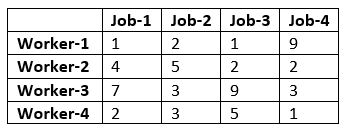
A manager has prepared a table that shows the cost of performing each of four jobs by each of four employees. The manager has stated his goal is to develop a set of job assignments that will minimize the total cost of getting all 4 jobs.
Initialize LP Model
In this step, we will import all the classes and functions of pulp module and create a Minimization LP problem using LpProblem class.
Define Decision Variable
In this step, we will define the decision variables. In our problem, we have two variable lists: workers and jobs. Let’s create them using LpVariable.dicts() class. LpVariable.dicts() used with Python’s list comprehension. LpVariable.dicts() will take the following four values:
- First, prefix name of what this variable represents.
- Second is the list of all the variables.
- Third is the lower bound on this variable.
- Fourth variable is the upper bound.
- Fourth is essentially the type of data (discrete or continuous). The options for the fourth parameter are LpContinuous or LpInteger .
Let’s first create a list route for the route between warehouse and project site and create the decision variables using LpVariable.dicts() the method.
Define Objective Function
In this step, we will define the minimum objective function by adding it to the LpProblem object. lpSum(vector)is used here to define multiple linear expressions. It also used list comprehension to add multiple variables.
Define the Constraints
Here, we are adding two types of constraints: Each job can be assigned to only one employee constraint and Each employee can be assigned to only one job. We have added the 2 constraints defined in the problem by adding them to the LpProblem object.
Solve Model
In this step, we will solve the LP problem by calling solve() method. We can print the final value by using the following for loop.
From the above results, we can infer that Worker-1 will be assigned to Job-1, Worker-2 will be assigned to job-3, Worker-3 will be assigned to Job-2, and Worker-4 will assign with job-4.
In this article, we have learned about Assignment problems, Problem Formulation, and implementation using the python PuLp library. We have solved the Assignment problem using a Linear programming problem in Python. Of course, this is just a simple case study, we can add more constraints to it and make it more complicated. You can also run other case studies on Cargo Loading problems , Staff scheduling problems . In upcoming articles, we will write more on different optimization problems such as transshipment problem, balanced diet problem. You can revise the basics of mathematical concepts in this article and learn about Linear Programming in this article .
- Solving Blending Problem in Python using Gurobi
- Transshipment Problem in Python Using PuLP
You May Also Like

DBSCAN Clustering

Text Analytics for Beginner using Python TextBlob

Pandas Series
scipy.optimize.quadratic_assignment #
Approximates solution to the quadratic assignment problem and the graph matching problem.
Quadratic assignment solves problems of the following form:
where \(\mathcal{P}\) is the set of all permutation matrices, and \(A\) and \(B\) are square matrices.
Graph matching tries to maximize the same objective function. This algorithm can be thought of as finding the alignment of the nodes of two graphs that minimizes the number of induced edge disagreements, or, in the case of weighted graphs, the sum of squared edge weight differences.
Note that the quadratic assignment problem is NP-hard. The results given here are approximations and are not guaranteed to be optimal.
The square matrix \(A\) in the objective function above.
The square matrix \(B\) in the objective function above.
The algorithm used to solve the problem. ‘faq’ (default) and ‘2opt’ are available.
A dictionary of solver options. All solvers support the following:
Maximizes the objective function if True .
Fixes part of the matching. Also known as a “seed” [2] .
Each row of partial_match specifies a pair of matched nodes: node partial_match[i, 0] of A is matched to node partial_match[i, 1] of B . The array has shape (m, 2) , where m is not greater than the number of nodes, \(n\) .
numpy.random.RandomState }, optional
If seed is None (or np.random ), the numpy.random.RandomState singleton is used. If seed is an int, a new RandomState instance is used, seeded with seed . If seed is already a Generator or RandomState instance then that instance is used.
For method-specific options, see show_options('quadratic_assignment') .
OptimizeResult containing the following fields.
Column indices corresponding to the best permutation found of the nodes of B .
The objective value of the solution.
The number of iterations performed during optimization.
The default method ‘faq’ uses the Fast Approximate QAP algorithm [1] ; it typically offers the best combination of speed and accuracy. Method ‘2opt’ can be computationally expensive, but may be a useful alternative, or it can be used to refine the solution returned by another method.
J.T. Vogelstein, J.M. Conroy, V. Lyzinski, L.J. Podrazik, S.G. Kratzer, E.T. Harley, D.E. Fishkind, R.J. Vogelstein, and C.E. Priebe, “Fast approximate quadratic programming for graph matching,” PLOS one, vol. 10, no. 4, p. e0121002, 2015, DOI:10.1371/journal.pone.0121002
D. Fishkind, S. Adali, H. Patsolic, L. Meng, D. Singh, V. Lyzinski, C. Priebe, “Seeded graph matching”, Pattern Recognit. 87 (2019): 203-215, DOI:10.1016/j.patcog.2018.09.014
“2-opt,” Wikipedia. https://en.wikipedia.org/wiki/2-opt
The see the relationship between the returned col_ind and fun , use col_ind to form the best permutation matrix found, then evaluate the objective function \(f(P) = trace(A^T P B P^T )\) .
Alternatively, to avoid constructing the permutation matrix explicitly, directly permute the rows and columns of the distance matrix.
Although not guaranteed in general, quadratic_assignment happens to have found the globally optimal solution.
Here is an example for which the default method, ‘faq’ , does not find the global optimum.
If accuracy is important, consider using ‘2opt’ to refine the solution.
Hungarian Algorithm Introduction & Python Implementation
How to use hungarian method to resolve the linear assignment problem..
By Eason on 2021-08-02
In this article, I will introduce how to use Hungarian Method to resolve the linear assignment problem and provide my personal Python code solution.
So… What is the linear assignment problem?
The linear assignment problem represents the need to maximize the available resources (or minimize the expenditure) with limited resources. For instance, below is a 2D matrix, where each row represents a different supplier, and each column represents the cost of employing them to produce a particular product. Each supplier can only specialize in the production of one of these products. In other words, only one element can be selected for each column and row in the matrix, and the sum of the selected elements must be minimized (minimized cost expense).
The cost of producing different goods by different producers:
Indeed, this is a simple example. By trying out the possible combinations, we can see that the smallest sum is 13, so supplier A supplies Bubble Tea , supplier B supplies milk tea, and supplier C supplies Fruit Tea . However, such attempts do not follow a clear rule and become inefficient when applied to large tasks. Therefore, the next section will introduce step by step the Hungarian algorithm, which can be applied to the linear assignment problem.
Hungarian Algorithm & Python Code Step by Step
In this section, we will show how to use the Hungarian algorithm to solve linear assignment problems and find the minimum combinations in the matrix. Of course, the Hungarian algorithm can also be used to find the maximum combination.
Step 0. Prepare Operations
First, an N by N matrix is generated to be used for the Hungarian algorithm (Here, we use a 5 by 5 square matrix as an example).
The above code randomly generates a 5x5 cost matrix of integers between 0 and 10.
If we want to find the maximum sum, we could do the opposite. The matrix to be solved is regarded as the profit matrix, and the maximum value in the matrix is set as the common price of all goods. The cost matrix is obtained by subtracting the profit matrix from the maximum value. Finally, the cost matrix is substituted into the Hungarian algorithm to obtain the minimized combination and then remapped back to the profit matrix to obtain the maximized sum value and composition result.
The above code randomly generates a 5x5 profit matrix of integers between 0 and 10 and generate a corresponding cost matrix
By following the steps above, you can randomly generate either the cost matrix or the profit matrix. Next, we will move into the introduction of the Hungarian algorithm, and for the sake of illustration, the following sections will be illustrated using the cost matrix shown below. We will use the Hungarian algorithm to solve the linear assignment problem of the cost matrix and find the corresponding minimum sum.
Example cost matrix:
Step 1. Every column and every row subtract its internal minimum
First, every column and every row must subtract its internal minimum. After subtracting the minimum, the cost matrix will look like this.
Cost matrix after step 1:
And the current code is like this:
Step 2.1. Min_zero_row Function Implementation
At first, we need to find the row with the fewest zero elements. So, we can convert the previous matrix to the boolean matrix(0 → True, Others → False).
Transform matrix to boolean matrix:
Corresponding Boolean matrix:
Therefore, we can use the “min_zero_row” function to find the corresponding row.
The row which contains the least 0:

Third, mark any 0 elements on the corresponding row and clean up its row and column (converts elements on the Boolean matrix to False). The coordinates of the element are stored in mark_zero.
Hence, the boolean matrix will look like this:
The boolean matrix after the first process. The fourth row has been changed to all False.
The process is repeated several times until the elements in the boolean matrix are all False. The below picture shows the order in which they are marked.
The possible answer composition:

Step 2.2. Mark_matrix Function Implementation
After getting Zero_mat from the step 2–1, we can check it and mark the matrix according to certain rules. The whole rule can be broken down into several steps:
- Mark rows that do not contain marked 0 elements and store row indexes in the non_marked_row
- Search non_marked_row element, and find out if there are any unmarked 0 elements in the corresponding column
- Store the column indexes in the marked_cols
- Compare the column indexes stored in marked_zero and marked_cols
- If a matching column index exists, the corresponding row_index is saved to non_marked_rows
- Next, the row indexes that are not in non_marked_row are stored in marked_rows
Finally, the whole mark_matrx function is finished and then returns marked_zero , marked_rows , marked_cols. At this point, we will be able to decide the result based on the return information.
If we use the example cost matrix, the corresponding marked_zero , marked_rows, and marked_cols are as follows:
- marked_zero : [(3, 2), (0, 4), (1, 1), (2, 0), (4, 3)]
- marked_rows : [0, 1, 2, 3, 4]
- marked_cols : []
Step 3. Identify the Result
At this step, if the sum of the lengths of marked_rows and marked_cols is equal to the length of the cost matrix, it means that the solution of the linear assignment problem has been found successfully, and marked_zero stores the solution coordinates. Fortunately, in the example matrix, we find the answer on the first try. Therefore, we can skip to step 5 and calculate the solution.
However, everything is hardly plain sailing. Most of the time, we will not find the solution on the first try, such as the following matrix:
After Step 1 & 2 , the corresponding matrix, marked_rows, and marked_cols are as follows:

The sum of the lengths of Marked_Rows and Marked_Cols is 4 (less than 5).
Apparently, the sum of the lengths is less than the length of the matrix. At this time, we need to go into Step 4 to adjust the matrix.
Step 4. Adjust Matrix
In Step 4, we're going to put the matrix after Step 1 into the Adjust_Matrix function . Taking the latter matrix in Step 3 as an example, the matrix to be modified in Adjust_Matrix is:
The whole function can be separated into three steps:
- Find the minimum value for an element that is not in marked_rows and not in marked_cols . Hence, we can find the minimum value is 1.

- Subtract the elements which not in marked_rows nor marked_cols from the minimum values obtained in the previous step.

- Add the element in marked_rows , which is also in marked_cols , to the minimum value obtained by Step 4–1.

Return the adjusted matrix and repeat Step 2 and Step 3 until the conditions satisfy the requirement of entering Step 5.
Step 5. Calculate the Answer
Using the element composition stored in marked_zero , the minimum and maximum values of the linear assignment problem can be calculated.

The minimum composition of the assigned matrix and the minimum sum is 18.

The maximum composition of the assigned matrix and the maximum sum is 43.
The code of the Answer_Calculator function is as follows:
The complete code is as follows:
Hungarian algorithm - Wikipedia
Continue Learning
How to read parquet files in python without a distributed cluster, how to use python to fetch phone number details, how to schedule recurring jobs or tasks using celery.
Schedule Jobs 2: Schedule recurring jobs/tasks using Celery.
How to Send Desktop Notifications with Python
No experience required!
22 Useful Snippets to Code like a Pro in Python
Why and how to write frozen dataclasses in python.
The difference between frozen and non-frozen dataclasses.

Hands-On Linear Programming: Optimization With Python
Table of Contents
What Is Linear Programming?
What is mixed-integer linear programming, why is linear programming important, linear programming with python, small linear programming problem, infeasible linear programming problem, unbounded linear programming problem, resource allocation problem, installing scipy and pulp, using scipy, linear programming resources, linear programming solvers.
Linear programming is a set of techniques used in mathematical programming , sometimes called mathematical optimization, to solve systems of linear equations and inequalities while maximizing or minimizing some linear function . It’s important in fields like scientific computing, economics, technical sciences, manufacturing, transportation, military, management, energy, and so on.
The Python ecosystem offers several comprehensive and powerful tools for linear programming. You can choose between simple and complex tools as well as between free and commercial ones. It all depends on your needs.
In this tutorial, you’ll learn:
- What linear programming is and why it’s important
- Which Python tools are suitable for linear programming
- How to build a linear programming model in Python
- How to solve a linear programming problem with Python
You’ll first learn about the fundamentals of linear programming. Then you’ll explore how to implement linear programming techniques in Python. Finally, you’ll look at resources and libraries to help further your linear programming journey.
Free Bonus: 5 Thoughts On Python Mastery , a free course for Python developers that shows you the roadmap and the mindset you’ll need to take your Python skills to the next level.
Linear Programming Explanation
In this section, you’ll learn the basics of linear programming and a related discipline, mixed-integer linear programming. In the next section , you’ll see some practical linear programming examples. Later, you’ll solve linear programming and mixed-integer linear programming problems with Python.
Imagine that you have a system of linear equations and inequalities. Such systems often have many possible solutions. Linear programming is a set of mathematical and computational tools that allows you to find a particular solution to this system that corresponds to the maximum or minimum of some other linear function.
Mixed-integer linear programming is an extension of linear programming. It handles problems in which at least one variable takes a discrete integer rather than a continuous value . Although mixed-integer problems look similar to continuous variable problems at first sight, they offer significant advantages in terms of flexibility and precision.
Integer variables are important for properly representing quantities naturally expressed with integers, like the number of airplanes produced or the number of customers served.
A particularly important kind of integer variable is the binary variable . It can take only the values zero or one and is useful in making yes-or-no decisions, such as whether a plant should be built or if a machine should be turned on or off. You can also use them to mimic logical constraints.
Linear programming is a fundamental optimization technique that’s been used for decades in science- and math-intensive fields. It’s precise, relatively fast, and suitable for a range of practical applications.
Mixed-integer linear programming allows you to overcome many of the limitations of linear programming. You can approximate non-linear functions with piecewise linear functions , use semi-continuous variables , model logical constraints, and more. It’s a computationally intensive tool, but the advances in computer hardware and software make it more applicable every day.
Often, when people try to formulate and solve an optimization problem, the first question is whether they can apply linear programming or mixed-integer linear programming.
Some use cases of linear programming and mixed-integer linear programming are illustrated in the following articles:
- Gurobi Optimization Case Studies
- Five Areas of Application for Linear Programming Techniques
The importance of linear programming, and especially mixed-integer linear programming, has increased over time as computers have gotten more capable, algorithms have improved, and more user-friendly software solutions have become available.
The basic method for solving linear programming problems is called the simplex method , which has several variants. Another popular approach is the interior-point method .
Mixed-integer linear programming problems are solved with more complex and computationally intensive methods like the branch-and-bound method , which uses linear programming under the hood. Some variants of this method are the branch-and-cut method , which involves the use of cutting planes , and the branch-and-price method .
There are several suitable and well-known Python tools for linear programming and mixed-integer linear programming. Some of them are open source, while others are proprietary. Whether you need a free or paid tool depends on the size and complexity of your problem as well as on the need for speed and flexibility.
It’s worth mentioning that almost all widely used linear programming and mixed-integer linear programming libraries are native to and written in Fortran or C or C++. This is because linear programming requires computationally intensive work with (often large) matrices. Such libraries are called solvers . The Python tools are just wrappers around the solvers.
Python is suitable for building wrappers around native libraries because it works well with C/C++. You’re not going to need any C/C++ (or Fortran) for this tutorial, but if you want to learn more about this cool feature, then check out the following resources:
- Building a Python C Extension Module
- CPython Internals
- Extending Python with C or C++
Basically, when you define and solve a model, you use Python functions or methods to call a low-level library that does the actual optimization job and returns the solution to your Python object.
Several free Python libraries are specialized to interact with linear or mixed-integer linear programming solvers:
- SciPy Optimization and Root Finding
In this tutorial, you’ll use SciPy and PuLP to define and solve linear programming problems.
Linear Programming Examples
In this section, you’ll see two examples of linear programming problems:
- A small problem that illustrates what linear programming is
- A practical problem related to resource allocation that illustrates linear programming concepts in a real-world scenario
You’ll use Python to solve these two problems in the next section .
Consider the following linear programming problem:
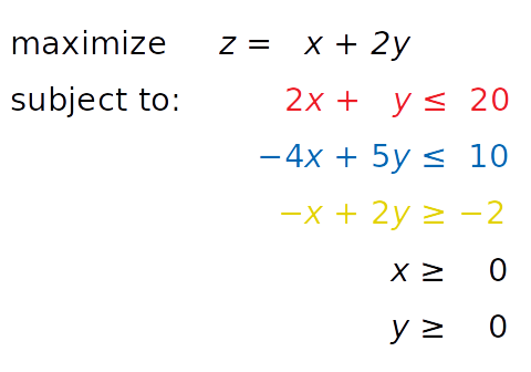
You need to find x and y such that the red, blue, and yellow inequalities, as well as the inequalities x ≥ 0 and y ≥ 0, are satisfied. At the same time, your solution must correspond to the largest possible value of z .
The independent variables you need to find—in this case x and y —are called the decision variables . The function of the decision variables to be maximized or minimized—in this case z —is called the objective function , the cost function , or just the goal . The inequalities you need to satisfy are called the inequality constraints . You can also have equations among the constraints called equality constraints .
This is how you can visualize the problem:
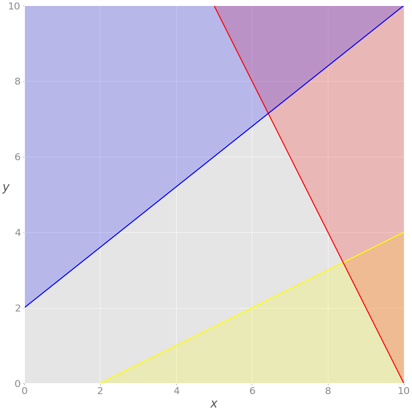
The red line represents the function 2 x + y = 20, and the red area above it shows where the red inequality is not satisfied. Similarly, the blue line is the function −4 x + 5 y = 10, and the blue area is forbidden because it violates the blue inequality. The yellow line is − x + 2 y = −2, and the yellow area below it is where the yellow inequality isn’t valid.
If you disregard the red, blue, and yellow areas, only the gray area remains. Each point of the gray area satisfies all constraints and is a potential solution to the problem. This area is called the feasible region , and its points are feasible solutions . In this case, there’s an infinite number of feasible solutions.
You want to maximize z . The feasible solution that corresponds to maximal z is the optimal solution . If you were trying to minimize the objective function instead, then the optimal solution would correspond to its feasible minimum.
Note that z is linear. You can imagine it as a plane in three-dimensional space. This is why the optimal solution must be on a vertex , or corner, of the feasible region. In this case, the optimal solution is the point where the red and blue lines intersect, as you’ll see later .
Sometimes a whole edge of the feasible region, or even the entire region, can correspond to the same value of z . In that case, you have many optimal solutions.
You’re now ready to expand the problem with the additional equality constraint shown in green:
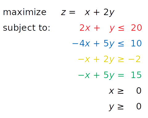
The equation − x + 5 y = 15, written in green, is new. It’s an equality constraint. You can visualize it by adding a corresponding green line to the previous image:
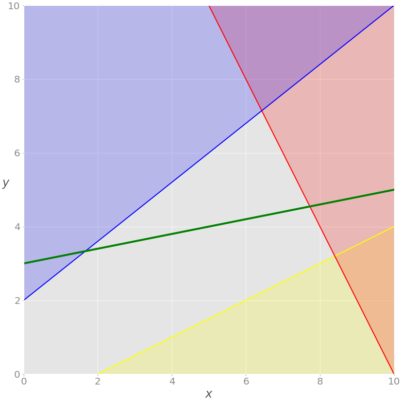
The solution now must satisfy the green equality, so the feasible region isn’t the entire gray area anymore. It’s the part of the green line passing through the gray area from the intersection point with the blue line to the intersection point with the red line. The latter point is the solution.
If you insert the demand that all values of x must be integers, then you’ll get a mixed-integer linear programming problem, and the set of feasible solutions will change once again:
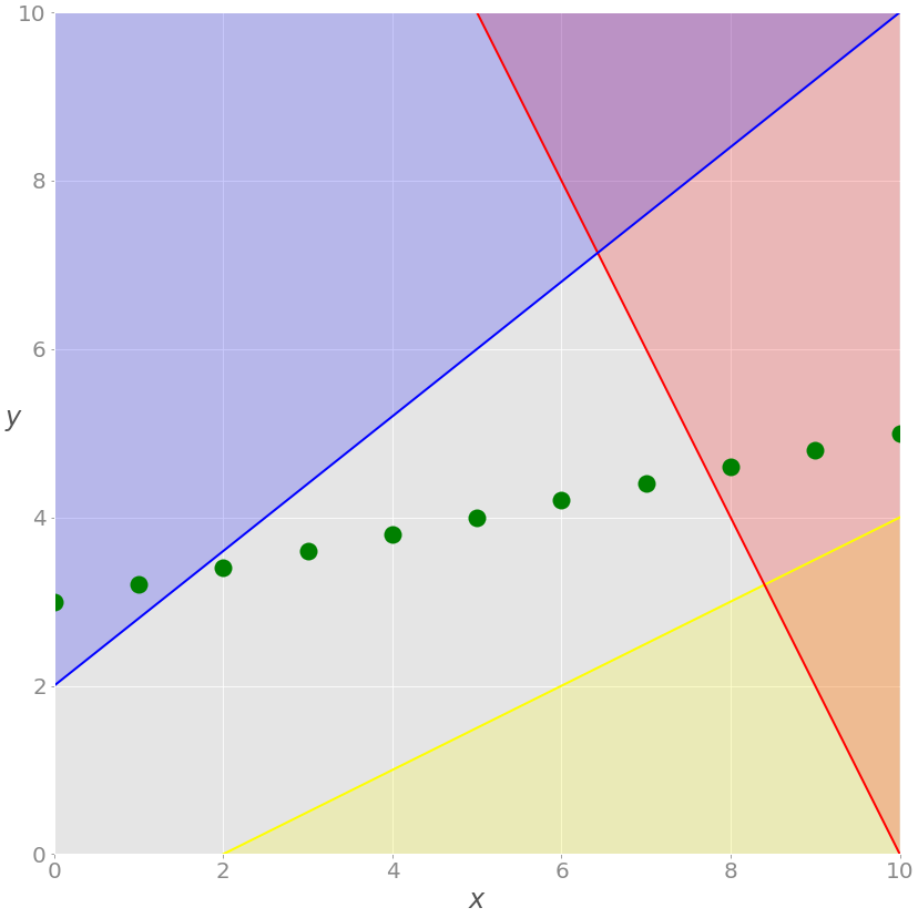
You no longer have the green line, only the points along the line where the value of x is an integer. The feasible solutions are the green points on the gray background, and the optimal one in this case is nearest to the red line.
These three examples illustrate feasible linear programming problems because they have bounded feasible regions and finite solutions.
A linear programming problem is infeasible if it doesn’t have a solution. This usually happens when no solution can satisfy all constraints at once.
For example, consider what would happen if you added the constraint x + y ≤ −1. Then at least one of the decision variables ( x or y ) would have to be negative. This is in conflict with the given constraints x ≥ 0 and y ≥ 0. Such a system doesn’t have a feasible solution, so it’s called infeasible.
Another example would be adding a second equality constraint parallel to the green line. These two lines wouldn’t have a point in common, so there wouldn’t be a solution that satisfies both constraints.
A linear programming problem is unbounded if its feasible region isn’t bounded and the solution is not finite. This means that at least one of your variables isn’t constrained and can reach to positive or negative infinity, making the objective infinite as well.
For example, say you take the initial problem above and drop the red and yellow constraints. Dropping constraints out of a problem is called relaxing the problem. In such a case, x and y wouldn’t be bounded on the positive side. You’d be able to increase them toward positive infinity, yielding an infinitely large z value.
In the previous sections, you looked at an abstract linear programming problem that wasn’t tied to any real-world application. In this subsection, you’ll find a more concrete and practical optimization problem related to resource allocation in manufacturing.
Say that a factory produces four different products, and that the daily produced amount of the first product is x ₁, the amount produced of the second product is x ₂, and so on. The goal is to determine the profit-maximizing daily production amount for each product, bearing in mind the following conditions:
The profit per unit of product is $20, $12, $40, and $25 for the first, second, third, and fourth product, respectively.
Due to manpower constraints, the total number of units produced per day can’t exceed fifty.
For each unit of the first product, three units of the raw material A are consumed. Each unit of the second product requires two units of the raw material A and one unit of the raw material B. Each unit of the third product needs one unit of A and two units of B. Finally, each unit of the fourth product requires three units of B.
Due to the transportation and storage constraints, the factory can consume up to one hundred units of the raw material A and ninety units of B per day.
The mathematical model can be defined like this:
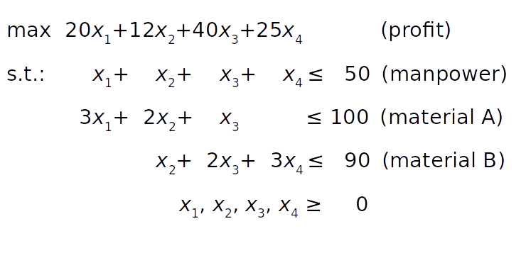
The objective function (profit) is defined in condition 1. The manpower constraint follows from condition 2. The constraints on the raw materials A and B can be derived from conditions 3 and 4 by summing the raw material requirements for each product.
Finally, the product amounts can’t be negative, so all decision variables must be greater than or equal to zero.
Unlike the previous example, you can’t conveniently visualize this one because it has four decision variables. However, the principles remain the same regardless of the dimensionality of the problem.
Linear Programming Python Implementation
In this tutorial, you’ll use two Python packages to solve the linear programming problem described above:
- SciPy is a general-purpose package for scientific computing with Python.
- PuLP is a Python linear programming API for defining problems and invoking external solvers.
SciPy is straightforward to set up. Once you install it, you’ll have everything you need to start. Its subpackage scipy.optimize can be used for both linear and nonlinear optimization .
PuLP allows you to choose solvers and formulate problems in a more natural way. The default solver used by PuLP is the COIN-OR Branch and Cut Solver (CBC) . It’s connected to the COIN-OR Linear Programming Solver (CLP) for linear relaxations and the COIN-OR Cut Generator Library (CGL) for cuts generation.
Another great open source solver is the GNU Linear Programming Kit (GLPK) . Some well-known and very powerful commercial and proprietary solutions are Gurobi , CPLEX , and XPRESS .
Besides offering flexibility when defining problems and the ability to run various solvers, PuLP is less complicated to use than alternatives like Pyomo or CVXOPT, which require more time and effort to master.
To follow this tutorial, you’ll need to install SciPy and PuLP. The examples below use version 1.4.1 of SciPy and version 2.1 of PuLP.
You can install both using pip :
You might need to run pulptest or sudo pulptest to enable the default solvers for PuLP, especially if you’re using Linux or Mac:
Optionally, you can download, install, and use GLPK. It’s free and open source and works on Windows, MacOS, and Linux. You’ll see how to use GLPK (in addition to CBC) with PuLP later in this tutorial.
On Windows, you can download the archives and run the installation files.
On MacOS, you can use Homebrew :
On Debian and Ubuntu, use apt to install glpk and glpk-utils :
On Fedora, use dnf with glpk-utils :
You might also find conda useful for installing GLPK:
After completing the installation, you can check the version of GLPK:
See GLPK’s tutorials on installing with Windows executables and Linux packages for more information.
In this section, you’ll learn how to use the SciPy optimization and root-finding library for linear programming.
To define and solve optimization problems with SciPy, you need to import scipy.optimize.linprog() :
Now that you have linprog() imported, you can start optimizing.
Let’s first solve the linear programming problem from above:
linprog() solves only minimization (not maximization) problems and doesn’t allow inequality constraints with the greater than or equal to sign (≥). To work around these issues, you need to modify your problem before starting optimization:
- Instead of maximizing z = x + 2 y, you can minimize its negative(− z = − x − 2 y).
- Instead of having the greater than or equal to sign, you can multiply the yellow inequality by −1 and get the opposite less than or equal to sign (≤).
After introducing these changes, you get a new system:
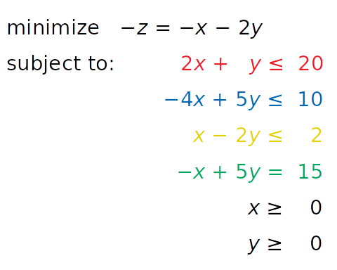
This system is equivalent to the original and will have the same solution. The only reason to apply these changes is to overcome the limitations of SciPy related to the problem formulation.
The next step is to define the input values:
You put the values from the system above into the appropriate lists, tuples , or NumPy arrays :
- obj holds the coefficients from the objective function.
- lhs_ineq holds the left-side coefficients from the inequality (red, blue, and yellow) constraints.
- rhs_ineq holds the right-side coefficients from the inequality (red, blue, and yellow) constraints.
- lhs_eq holds the left-side coefficients from the equality (green) constraint.
- rhs_eq holds the right-side coefficients from the equality (green) constraint.
Note: Please, be careful with the order of rows and columns!
The order of the rows for the left and right sides of the constraints must be the same. Each row represents one constraint.
The order of the coefficients from the objective function and left sides of the constraints must match. Each column corresponds to a single decision variable.
The next step is to define the bounds for each variable in the same order as the coefficients. In this case, they’re both between zero and positive infinity:
This statement is redundant because linprog() takes these bounds (zero to positive infinity) by default.
Note: Instead of float("inf") , you can use math.inf , numpy.inf , or scipy.inf .
Finally, it’s time to optimize and solve your problem of interest. You can do that with linprog() :
The parameter c refers to the coefficients from the objective function. A_ub and b_ub are related to the coefficients from the left and right sides of the inequality constraints, respectively. Similarly, A_eq and b_eq refer to equality constraints. You can use bounds to provide the lower and upper bounds on the decision variables.
You can use the parameter method to define the linear programming method that you want to use. There are three options:
- method="interior-point" selects the interior-point method. This option is set by default.
- method="revised simplex" selects the revised two-phase simplex method.
- method="simplex" selects the legacy two-phase simplex method.
linprog() returns a data structure with these attributes:
.con is the equality constraints residuals.
.fun is the objective function value at the optimum (if found).
.message is the status of the solution.
.nit is the number of iterations needed to finish the calculation.
.slack is the values of the slack variables, or the differences between the values of the left and right sides of the constraints.
.status is an integer between 0 and 4 that shows the status of the solution, such as 0 for when the optimal solution has been found.
.success is a Boolean that shows whether the optimal solution has been found.
.x is a NumPy array holding the optimal values of the decision variables.
You can access these values separately:
That’s how you get the results of optimization. You can also show them graphically:
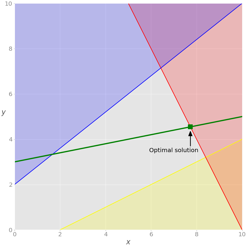
As discussed earlier, the optimal solutions to linear programming problems lie at the vertices of the feasible regions. In this case, the feasible region is just the portion of the green line between the blue and red lines. The optimal solution is the green square that represents the point of intersection between the green and red lines.
If you want to exclude the equality (green) constraint, just drop the parameters A_eq and b_eq from the linprog() call:
The solution is different from the previous case. You can see it on the chart:
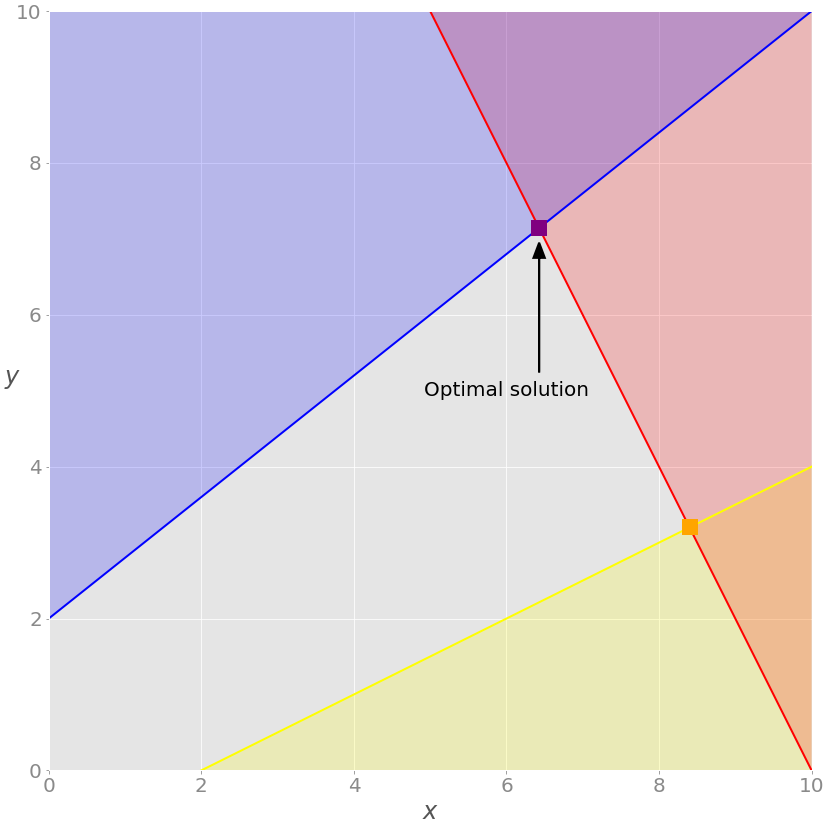
In this example, the optimal solution is the purple vertex of the feasible (gray) region where the red and blue constraints intersect. Other vertices, like the yellow one, have higher values for the objective function.
You can use SciPy to solve the resource allocation problem stated in the earlier section :
As in the previous example, you need to extract the necessary vectors and matrix from the problem above, pass them as the arguments to .linprog() , and get the results:
The result tells you that the maximal profit is 1900 and corresponds to x ₁ = 5 and x ₃ = 45. It’s not profitable to produce the second and fourth products under the given conditions. You can draw several interesting conclusions here:
The third product brings the largest profit per unit, so the factory will produce it the most.
The first slack is 0 , which means that the values of the left and right sides of the manpower (first) constraint are the same. The factory produces 50 units per day, and that’s its full capacity.
The second slack is 40 because the factory consumes 60 units of raw material A (15 units for the first product plus 45 for the third) out of a potential 100 units.
The third slack is 0 , which means that the factory consumes all 90 units of the raw material B. This entire amount is consumed for the third product. That’s why the factory can’t produce the second or fourth product at all and can’t produce more than 45 units of the third product. It lacks the raw material B.
opt.status is 0 and opt.success is True , indicating that the optimization problem was successfully solved with the optimal feasible solution.
SciPy’s linear programming capabilities are useful mainly for smaller problems. For larger and more complex problems, you might find other libraries more suitable for the following reasons:
SciPy can’t run various external solvers.
SciPy can’t work with integer decision variables.
SciPy doesn’t provide classes or functions that facilitate model building. You have to define arrays and matrices, which might be a tedious and error-prone task for large problems.
SciPy doesn’t allow you to define maximization problems directly. You must convert them to minimization problems.
SciPy doesn’t allow you to define constraints using the greater-than-or-equal-to sign directly. You must use the less-than-or-equal-to instead.
Fortunately, the Python ecosystem offers several alternative solutions for linear programming that are very useful for larger problems. One of them is PuLP, which you’ll see in action in the next section.
PuLP has a more convenient linear programming API than SciPy. You don’t have to mathematically modify your problem or use vectors and matrices. Everything is cleaner and less prone to errors.
As usual, you start by importing what you need:
Now that you have PuLP imported, you can solve your problems.
You’ll now solve this system with PuLP:
The first step is to initialize an instance of LpProblem to represent your model:
You use the sense parameter to choose whether to perform minimization ( LpMinimize or 1 , which is the default) or maximization ( LpMaximize or -1 ). This choice will affect the result of your problem.
Once that you have the model, you can define the decision variables as instances of the LpVariable class:
You need to provide a lower bound with lowBound=0 because the default value is negative infinity. The parameter upBound defines the upper bound, but you can omit it here because it defaults to positive infinity.
The optional parameter cat defines the category of a decision variable. If you’re working with continuous variables, then you can use the default value "Continuous" .
You can use the variables x and y to create other PuLP objects that represent linear expressions and constraints:
When you multiply a decision variable with a scalar or build a linear combination of multiple decision variables, you get an instance of pulp.LpAffineExpression that represents a linear expression.
Note: You can add or subtract variables or expressions, and you can multiply them with constants because PuLP classes implement some of the Python special methods that emulate numeric types like __add__() , __sub__() , and __mul__() . These methods are used to customize the behavior of operators like + , - , and * .
Similarly, you can combine linear expressions, variables, and scalars with the operators == , <= , or >= to get instances of pulp.LpConstraint that represent the linear constraints of your model.
Note: It’s also possible to build constraints with the rich comparison methods .__eq__() , .__le__() , and .__ge__() that define the behavior of the operators == , <= , and >= .
Having this in mind, the next step is to create the constraints and objective function as well as to assign them to your model. You don’t need to create lists or matrices. Just write Python expressions and use the += operator to append them to the model:
In the above code, you define tuples that hold the constraints and their names. LpProblem allows you to add constraints to a model by specifying them as tuples. The first element is a LpConstraint instance. The second element is a human-readable name for that constraint.
Setting the objective function is very similar:
Alternatively, you can use a shorter notation:
Now you have the objective function added and the model defined.
Note: You can append a constraint or objective to the model with the operator += because its class, LpProblem , implements the special method .__iadd__() , which is used to specify the behavior of += .
For larger problems, it’s often more convenient to use lpSum() with a list or other sequence than to repeat the + operator. For example, you could add the objective function to the model with this statement:
It produces the same result as the previous statement.
You can now see the full definition of this model:
The string representation of the model contains all relevant data: the variables, constraints, objective, and their names.
Note: String representations are built by defining the special method .__repr__() . For more details about .__repr__() , check out Pythonic OOP String Conversion: __repr__ vs __str__ or When Should You Use .__repr__() vs .__str__() in Python? .
Finally, you’re ready to solve the problem. You can do that by calling .solve() on your model object. If you want to use the default solver (CBC), then you don’t need to pass any arguments:
.solve() calls the underlying solver, modifies the model object, and returns the integer status of the solution, which will be 1 if the optimum is found. For the rest of the status codes, see LpStatus[] .
You can get the optimization results as the attributes of model . The function value() and the corresponding method .value() return the actual values of the attributes:
model.objective holds the value of the objective function, model.constraints contains the values of the slack variables, and the objects x and y have the optimal values of the decision variables. model.variables() returns a list with the decision variables:
As you can see, this list contains the exact objects that are created with the constructor of LpVariable .
The results are approximately the same as the ones you got with SciPy.
Note: Be careful with the method .solve() —it changes the state of the objects x and y !
You can see which solver was used by calling .solver :
The output informs you that the solver is CBC. You didn’t specify a solver, so PuLP called the default one.
If you want to run a different solver, then you can specify it as an argument of .solve() . For example, if you want to use GLPK and already have it installed, then you can use solver=GLPK(msg=False) in the last line. Keep in mind that you’ll also need to import it:
Now that you have GLPK imported, you can use it inside .solve() :
The msg parameter is used to display information from the solver. msg=False disables showing this information. If you want to include the information, then just omit msg or set msg=True .
Your model is defined and solved, so you can inspect the results the same way you did in the previous case:
You got practically the same result with GLPK as you did with SciPy and CBC.
Let’s peek and see which solver was used this time:
As you defined above with the highlighted statement model.solve(solver=GLPK(msg=False)) , the solver is GLPK.
You can also use PuLP to solve mixed-integer linear programming problems. To define an integer or binary variable, just pass cat="Integer" or cat="Binary" to LpVariable . Everything else remains the same:
In this example, you have one integer variable and get different results from before:
Now x is an integer, as specified in the model. (Technically it holds a float value with zero after the decimal point.) This fact changes the whole solution. Let’s show this on the graph:
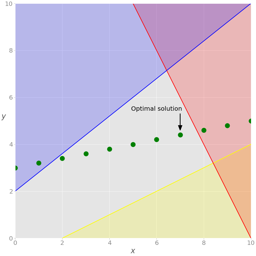
As you can see, the optimal solution is the rightmost green point on the gray background. This is the feasible solution with the largest values of both x and y , giving it the maximal objective function value.
GLPK is capable of solving such problems as well.
Now you can use PuLP to solve the resource allocation problem from above:
The approach for defining and solving the problem is the same as in the previous example:
In this case, you use the dictionary x to store all decision variables. This approach is convenient because dictionaries can store the names or indices of decision variables as keys and the corresponding LpVariable objects as values. Lists or tuples of LpVariable instances can be useful as well.
The code above produces the following result:
As you can see, the solution is consistent with the one obtained using SciPy. The most profitable solution is to produce 5.0 units of the first product and 45.0 units of the third product per day.
Let’s make this problem more complicated and interesting. Say the factory can’t produce the first and third products in parallel due to a machinery issue. What’s the most profitable solution in this case?
Now you have another logical constraint: if x ₁ is positive, then x ₃ must be zero and vice versa. This is where binary decision variables are very useful. You’ll use two binary decision variables, y ₁ and y ₃, that’ll denote if the first or third products are generated at all:
The code is very similar to the previous example except for the highlighted lines. Here are the differences:
Line 5 defines the binary decision variables y[1] and y[3] held in the dictionary y .
Line 12 defines an arbitrarily large number M . The value 100 is large enough in this case because you can’t have more than 100 units per day.
Line 13 says that if y[1] is zero, then x[1] must be zero, else it can be any non-negative number.
Line 14 says that if y[3] is zero, then x[3] must be zero, else it can be any non-negative number.
Line 15 says that either y[1] or y[3] is zero (or both are), so either x[1] or x[3] must be zero as well.
Here’s the solution:
It turns out that the optimal approach is to exclude the first product and to produce only the third one.
Linear programming and mixed-integer linear programming are very important topics. If you want to learn more about them—and there’s much more to learn than what you saw here—then you can find plenty of resources. Here are a few to get started with:
- Wikipedia Linear Programming Article
- Wikipedia Integer Programming Article
- MIT Introduction to Mathematical Programming Course
- Brilliant.org Linear Programming Article
- CalcWorkshop What Is Linear Programming?
- BYJU’S Linear Programming Article
Gurobi Optimization is a company that offers a very fast commercial solver with a Python API. It also provides valuable resources on linear programming and mixed-integer linear programming, including the following:
- Linear Programming (LP) – A Primer on the Basics
- Mixed-Integer Programming (MIP) – A Primer on the Basics
- Choosing a Math Programming Solver
If you’re in the mood to learn optimization theory, then there’s plenty of math books out there. Here are a few popular choices:
- Linear Programming: Foundations and Extensions
- Convex Optimization
- Model Building in Mathematical Programming
- Engineering Optimization: Theory and Practice
This is just a part of what’s available. Linear programming and mixed-integer linear programming are popular and widely used techniques, so you can find countless resources to help deepen your understanding.
Just like there are many resources to help you learn linear programming and mixed-integer linear programming, there’s also a wide range of solvers that have Python wrappers available. Here’s a partial list:
- SCIP with PySCIPOpt
- Gurobi Optimizer
Some of these libraries, like Gurobi, include their own Python wrappers. Others use external wrappers. For example, you saw that you can access CBC and GLPK with PuLP.
You now know what linear programming is and how to use Python to solve linear programming problems. You also learned that Python linear programming libraries are just wrappers around native solvers. When the solver finishes its job, the wrapper returns the solution status, the decision variable values, the slack variables, the objective function, and so on.
In this tutorial, you learned how to:
- Define a model that represents your problem
- Create a Python program for optimization
- Run the optimization program to find the solution to the problem
- Retrieve the result of optimization
You used SciPy with its own solver as well as PuLP with CBC and GLPK, but you also learned that there are many other linear programming solvers and Python wrappers. You’re now ready to dive into the world of linear programming!
If you have any questions or comments, then please put them in the comments section below.
🐍 Python Tricks 💌
Get a short & sweet Python Trick delivered to your inbox every couple of days. No spam ever. Unsubscribe any time. Curated by the Real Python team.

About Mirko Stojiljković

Mirko has a Ph.D. in Mechanical Engineering and works as a university professor. He is a Pythonista who applies hybrid optimization and machine learning methods to support decision making in the energy sector.
Each tutorial at Real Python is created by a team of developers so that it meets our high quality standards. The team members who worked on this tutorial are:

Master Real-World Python Skills With Unlimited Access to Real Python
Join us and get access to thousands of tutorials, hands-on video courses, and a community of expert Pythonistas:
Join us and get access to thousands of tutorials, hands-on video courses, and a community of expert Pythonistas:
What Do You Think?
What’s your #1 takeaway or favorite thing you learned? How are you going to put your newfound skills to use? Leave a comment below and let us know.
Commenting Tips: The most useful comments are those written with the goal of learning from or helping out other students. Get tips for asking good questions and get answers to common questions in our support portal . Looking for a real-time conversation? Visit the Real Python Community Chat or join the next “Office Hours” Live Q&A Session . Happy Pythoning!
Keep Learning
Related Topics: intermediate data-science
Keep reading Real Python by creating a free account or signing in:
Already have an account? Sign-In
Almost there! Complete this form and click the button below to gain instant access:

5 Thoughts On Python Mastery
🔒 No spam. We take your privacy seriously.

- Google OR-Tools
- Español – América Latina
- Português – Brasil
- Tiếng Việt
Linear Sum Assignment Solver
This section describes the linear sum assignment solver , a specialized solver for the simple assignment problem, which can be faster than either the MIP or CP-SAT solver. However, the MIP and CP-SAT solvers can handle a much wider array of problems, so in most cases they are the best option.
Cost matrix
The costs for workers and task are given in the table below.
| Worker | Task 0 | Task 1 | Task 2 | Task 3 |
|---|---|---|---|---|
| 90 | 76 | 75 | 70 | |
| 35 | 85 | 55 | 65 | |
| 125 | 95 | 90 | 105 | |
| 45 | 110 | 95 | 115 |
The following sections present a Python program that solves an assignment problem using the linear sum assignment solver.
Import the libraries
The code that imports the required library is shown below.
Define the data
The following code creates the data for the program.
The array is the cost matrix , whose i , j entry is the cost for worker i to perform task j . There are four workers, corresponding to the rows of the matrix, and four tasks, corresponding to the columns.
Create the solver
The program uses the linear assignment solver, a specialized solver for the assignment problem.
The following code creates the solver.
Add the constraints
The following code adds the costs to the solver by looping over workers and tasks.
Invoke the solver
The following code invokes the solver.
Display the results
The following code displays the solution.
The output below shows the optimal assignment of workers to tasks.
The following graph shows the solution as the dashed edges in the graph. The numbers next to the dashed edges are their costs. The total wait time of this assignment is the sum of the costs for the dashed edges, which is 265.
In graph theory, a set of edges in a bipartite graph that matches every node on the left with exactly one node on the right is called a perfect matching .
The entire program
Here is the entire program.
Solution when workers can't perform all tasks
In the previous example, we assumed that all workers can perform all tasks. But this not always the case - a worker might be unable to perform one or more tasks for various reasons. However, it is easy to modify the program above to handle this.
As an example, suppose that worker 0 is unable to perform task 3. To modify the program to take this into account, make the following changes:
- Change the 0, 3 entry of the cost matrix to the string 'NA' . (Any string will work.) cost = [[90, 76, 75, 'NA'], [35, 85, 55, 65], [125, 95, 90, 105], [45, 110, 95, 115]]
- In the section of the code that assigns costs to the solver, add the line if cost[worker][task] != 'NA': , as shown below. for worker in range(0, rows): for task in range(0, cols): if cost[worker][task] != 'NA': assignment.AddArcWithCost(worker, task, cost[worker][task]) The added line prevents any edge whose entry in the cost matrix is 'NA' from being added to the solver.
After making these changes and running the modified code, you see the following output:
Notice that the total cost is higher now than it was for the original problem. This is not surprising, since in the original problem the optimal solution assigned worker 0 to task 3, while in the modified problem that assignment is not allowed.
To see what happens if more workers are unable to perform tasks, you can replace more entries of the cost matrix with 'NA' , to denote additional workers who can't perform certain tasks:
When you run the program this time, you get a negative result:
This means there is no way to assign workers to tasks so that each worker performs a different task. You can see why this is so by looking at the graph for the problem (in which there are no edges corresponding to values of 'NA' in the cost matrix).
Since the nodes for the three workers 0, 1, and 2 are only connected to the two nodes for tasks 0 and 1, it not possible to assign distinct tasks to these workers.
The Marriage Theorem
There is a well-known result in graph theory, called The Marriage Theorem , which tells us exactly when you can assign each node on the left to a distinct node on the right, in a bipartite graph like the one above. Such an assignment is called a perfect matching . In a nutshell, the theorem says this is possible if there is no subset of nodes on the left (like the one in the previous example ) whose edges lead to a smaller set of nodes on the right.
More precisely, the theorem says that a bipartite graph has a perfect matching if and only if for any subset S of the nodes on the left side of the graph, the set of nodes on the right side of the graph that are connected by an edge to a node in S is at least as large as S.
Except as otherwise noted, the content of this page is licensed under the Creative Commons Attribution 4.0 License , and code samples are licensed under the Apache 2.0 License . For details, see the Google Developers Site Policies . Java is a registered trademark of Oracle and/or its affiliates.
Last updated 2023-01-18 UTC.
Learn Python practically and Get Certified .
Popular Tutorials
Popular examples, reference materials, learn python interactively, python introduction.
- Get Started With Python
- Your First Python Program
- Python Comments
Python Fundamentals
- Python Variables and Literals
- Python Type Conversion
- Python Basic Input and Output
- Python Operators
Python Flow Control
- Python if...else Statement
- Python for Loop
- Python while Loop
- Python break and continue
- Python pass Statement
Python Data types
- Python Numbers and Mathematics
- Python List
- Python Tuple
- Python String
- Python Sets
- Python Dictionary
- Python Functions
- Python Function Arguments
- Python Variable Scope
- Python Global Keyword
- Python Recursion
- Python Modules
- Python Package
- Python Main function

Python Files
- Python Directory and Files Management
- Python CSV: Read and Write CSV files
- Reading CSV files in Python
- Writing CSV files in Python
- Python Exception Handling
- Python Exceptions
- Python Custom Exceptions
Python Object & Class
- Python Objects and Classes
- Python Inheritance
- Python Multiple Inheritance
- Polymorphism in Python
- Python Operator Overloading
Python Advanced Topics
- List comprehension
- Python Lambda/Anonymous Function
- Python Iterators
- Python Generators
- Python Namespace and Scope
- Python Closures
- Python Decorators
- Python @property decorator
- Python RegEx
Python Date and Time
- Python datetime
- Python strftime()
- Python strptime()
- How to get current date and time in Python?
- Python Get Current Time
- Python timestamp to datetime and vice-versa
- Python time Module
- Python sleep()
Additional Topic
- Precedence and Associativity of Operators in Python
- Python Keywords and Identifiers
- Python Asserts
- Python Json
- Python *args and **kwargs
Python Tutorials
Python Array
Python List copy()
Python Shallow Copy and Deep Copy
- Python abs()
- Python List Comprehension
Python Matrices and NumPy Arrays
A matrix is a two-dimensional data structure where numbers are arranged into rows and columns. For example:
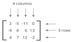
This matrix is a 3x4 (pronounced "three by four") matrix because it has 3 rows and 4 columns.
- Python Matrix
Python doesn't have a built-in type for matrices. However, we can treat a list of a list as a matrix. For example:
We can treat this list of a list as a matrix having 2 rows and 3 columns.

Be sure to learn about Python lists before proceed this article.
Let's see how to work with a nested list.
When we run the program, the output will be:
Here are few more examples related to Python matrices using nested lists.
- Add two matrices
- Transpose a Matrix
- Multiply two matrices
Using nested lists as a matrix works for simple computational tasks, however, there is a better way of working with matrices in Python using NumPy package.
- NumPy Array
NumPy is a package for scientific computing which has support for a powerful N-dimensional array object. Before you can use NumPy, you need to install it. For more info,
- Visit: How to install NumPy?
- If you are on Windows, download and install anaconda distribution of Python. It comes with NumPy and other several packages related to data science and machine learning.
Once NumPy is installed, you can import and use it.
NumPy provides multidimensional array of numbers (which is actually an object). Let's take an example:
As you can see, NumPy's array class is called ndarray .
How to create a NumPy array?
There are several ways to create NumPy arrays.
1. Array of integers, floats and complex Numbers
When you run the program, the output will be:
2. Array of zeros and ones
Here, we have specified dtype to 32 bits (4 bytes). Hence, this array can take values from -2 -31 to 2 -31 -1 .
3. Using arange() and shape()
Learn more about other ways of creating a NumPy array .
Matrix Operations
Above, we gave you 3 examples: addition of two matrices, multiplication of two matrices and transpose of a matrix. We used nested lists before to write those programs. Let's see how we can do the same task using NumPy array.
Addition of Two Matrices
We use + operator to add corresponding elements of two NumPy matrices.
Multiplication of Two Matrices
To multiply two matrices, we use dot() method. Learn more about how numpy.dot works.
Note: * is used for array multiplication (multiplication of corresponding elements of two arrays) not matrix multiplication.
Transpose of a Matrix
We use numpy.transpose to compute transpose of a matrix.
As you can see, NumPy made our task much easier.
Access matrix elements, rows and columns
Access matrix elements
Similar like lists, we can access matrix elements using index. Let's start with a one-dimensional NumPy array.
Now, let's see how we can access elements of a two-dimensional array (which is basically a matrix).
Access rows of a Matrix
Access columns of a Matrix
If you don't know how this above code works, read slicing of a matrix section of this article.
Slicing of a Matrix
Slicing of a one-dimensional NumPy array is similar to a list. If you don't know how slicing for a list works, visit Understanding Python's slice notation .
Let's take an example:
Now, let's see how we can slice a matrix.
As you can see, using NumPy (instead of nested lists) makes it a lot easier to work with matrices, and we haven't even scratched the basics. We suggest you to explore NumPy package in detail especially if you trying to use Python for data science/analytics.
NumPy Resources you might find helpful:
- NumPy Tutorial
- NumPy Reference
Table of Contents
- What is a matrix?
- Numbers(integers, float, complex etc.) Array
- Zeros and Ones Array
- Array Using arange() and shape()
- Multiplication
- Access elements
- Access rows
- Access columns
- Slicing of Matrix
- Useful Resources
Sorry about that.
Related Tutorials
Python Tutorial
Python Library
Navigation Menu
Search code, repositories, users, issues, pull requests..., provide feedback.
We read every piece of feedback, and take your input very seriously.
Saved searches
Use saved searches to filter your results more quickly.
To see all available qualifiers, see our documentation .
assignment-problem
Here are 22 public repositories matching this topic..., root-11 / graph-theory.
A simple graph library
- Updated Apr 29, 2024
mayorx / hungarian-algorithm
(Kuhn-Munkres) numpy implementation, rectangular matrix is supported (|X| <= |Y|). 100x100000 in 0.153 s.
- Updated Dec 8, 2022
sharathadavanne / hungarian-net
Deep-learning-based implementation of the popular Hungarian algorithm that helps solve the assignment problem.
- Updated Aug 31, 2023
YaleDHLab / pointgrid
Transform a 2D point distribution to a hex grid to avoid overplotting in data visualizations
- Updated Jun 30, 2021
dutta-alankar / PH-354-2019-IISc-Assignment-Problems
Solutions to the complete set of assignment problems which I did while crediting Computational Physics course by Prof. Manish Jain at IISc, Physical Sciences department on 2019
- Updated May 30, 2021
Ibrahim5aad / kuhn-munkres-algorithm
A python program to solve assignment problem by the Kuhn–Munkres algorithm (The Hungarian Method).
- Updated Oct 22, 2021
alierenekinci / SoforAtama
Driver Assignment WebUi
- Updated Jan 14, 2024
kachark / FormFlight
Simulation framework for autonomous vehicle formation and assignment
- Updated Oct 30, 2021
dilsonpereira / BipartiteMatching
Python implementation of algorithms for maximum cardinality matching and maximum cost assignment in bipartite graphs
- Updated Jul 25, 2019
swetanksaha / cse4589-pa3
AutoGrader & Student Template for the CSE 4/589: Programming Assignment 3 (PA3) [For use by TA & Course Instructors]
- Updated Jan 21, 2018
torressa / glovo
Some work I did for an interview for a job as a data scientist optimisation specialist
- Updated Jul 22, 2020
swetanksaha / cse4589-pa1
AutoGrader & Student Template for the CSE 4/589: Programming Assignment 1 (PA1) [For use by TA & Course Instructors]
- Updated Jan 23, 2019
asujaykk / MultiObjectTracker
An object tracker for realtime multiple objects tracking
- Updated Jan 9, 2023
zhiao777774 / task-assignment-tool
- Updated Nov 21, 2022
castroisabel / assignment-problem
Two different solutions for the assignment problem using the GLPK solver and the greedy algorithm.
- Updated Jan 1, 2022
calcoloergosum / assignment-enumeration-python
- Updated Jun 7, 2021
Iwilsonp / stable-scioly-team-assigner
- Updated Jan 30, 2018
simranjeet97 / RecyclingMachine
Python Recycling Machine Based on OOPS Concepts.
- Updated Feb 8, 2019
mridulgain / spyder
Simple Python Debugger
- Updated Jan 26, 2020
bornabr / assignment-problem-ant-colony
- Updated Dec 4, 2021
Improve this page
Add a description, image, and links to the assignment-problem topic page so that developers can more easily learn about it.
Curate this topic
Add this topic to your repo
To associate your repository with the assignment-problem topic, visit your repo's landing page and select "manage topics."
- Stack Overflow Public questions & answers
- Stack Overflow for Teams Where developers & technologists share private knowledge with coworkers
- Talent Build your employer brand
- Advertising Reach developers & technologists worldwide
- Labs The future of collective knowledge sharing
- About the company
Collectives™ on Stack Overflow
Find centralized, trusted content and collaborate around the technologies you use most.
Q&A for work
Connect and share knowledge within a single location that is structured and easy to search.
Get early access and see previews of new features.
Unbalanced worker/machine assignment
I have a problem of assigning 7 possible workers to 3 machines. There is a cost when a worker is assigned to a machine as well as when a worker is idle. It is required that all 3 machines are used. The cost matrices are
With matrix C being the cost of each worker being assigned to each machine. Matrix I represents the cost of each worker to be idle.
I'm currently using scipy.optimize.linear_sum_assignment to determine the minimum cost with a cost matrix
With the current cost matrix it sometimes happens that not all machines are assigned. To counter this I simply multiplied all the idle cost with 10 to ensure that the machines are selected first.
My python code however does not give me the optimal answer. Is there maybe a different function I could use that would solves this type of problems?
I need a way to solve the assignment while forcing all three the machines to be assigned a worker. My way of defining the cost matrix seems to do it but doesn't give the wanted answer (obtained using a Tabu search). I'm not sure how to force scipy.optimize.linear_sum_assignment to always assign the three machines. Is this even possible to do in scipy.optimize.linear_sum_assignment or should I rather be for a different python package to use?
- variable-assignment
- My python code however does not give me the optimal answer How can we possibly help if you don't show us the code? – John Gordon Commented Aug 29, 2016 at 21:02
- Welcome to StackOverflow. Please read and follow the posting guidelines in the help documentation. Minimal, complete, verifiable example applies here. We cannot effectively help you until you post your code and accurately describe the problem. – Prune Commented Aug 29, 2016 at 21:09
Found what was wrong with it. I had to many dummy machines allowing workers to be assigned to them rather than to the machines. By changing the dimensions of the matrix to be square (7x7) and changing the cost matrix
scipy.optimize.linear_sum_assignment now gives me the correct assignment.
Your Answer
Reminder: Answers generated by artificial intelligence tools are not allowed on Stack Overflow. Learn more
Sign up or log in
Post as a guest.
Required, but never shown
By clicking “Post Your Answer”, you agree to our terms of service and acknowledge you have read our privacy policy .
Not the answer you're looking for? Browse other questions tagged python matrix variable-assignment or ask your own question .
- Featured on Meta
- Upcoming sign-up experiments related to tags
- Policy: Generative AI (e.g., ChatGPT) is banned
- The return of Staging Ground to Stack Overflow
- The 2024 Developer Survey Is Live
Hot Network Questions
- If I'm using HSTS, can I skip the scheme from my CSP directives?
- Why are heavy metals toxic? Lead and Carbon are in the same group. One is toxic, the other is not
- What is the use in arguing for or against the existence of metaphysical things?
- How (if at all) are the PHB rules on Hiding affected by the Skulker feat and the Mask of the Wild trait?
- Is there any way to play Runescape singleplayer?
- If "Good luck finding a new job" is sarcastic, how do change the sentence to make it sound well-intentioned?
- Lufthansa bus no-show
- How do regression loss functions like MAE and MSE work although they remove the plus/minus sign?
- How can the CMOS version of 555 timer have the output current tested at 2 mA while its maximum supply is 250 μA?
- Why are amber bottles used to store Water for HPLC?
- Does it matter to de-select faces before going back to Object Mode?
- Short story crashing landing on a planet and taking shelter in a building that had automated defenses
- Movie with a gate guarded by two statues
- Replacing grass against side of house
- The term 'sfp' is not recognized
- Reviewers do not live up to own quality standards
- What is the difference between "боля" and "болея"?
- Am I getting scammed
- Is there any piece that can take multiple pieces at once?
- What is this biplane seen over Doncaster?
- Geographic distribution of Bitcoin users
- What is the relevance and meaning if a sentence contains "Had not"?
- Animated series about a tribe searching for a utopia with a kid who is different from the rest of them
- How did the `long` and `short` integer types originate?
- Data Structures
- Linked List
- Binary Tree
- Binary Search Tree
- Segment Tree
- Disjoint Set Union
- Fenwick Tree
- Red-Black Tree
- Advanced Data Structures
Hungarian Algorithm for Assignment Problem | Set 2 (Implementation)
- Hungarian Algorithm for Assignment Problem | Set 1 (Introduction)
- Implementation of Exhaustive Search Algorithm for Set Packing
- Greedy Approximate Algorithm for Set Cover Problem
- Introduction to Exact Cover Problem and Algorithm X
- Job Assignment Problem using Branch And Bound
- Prim's Algorithm (Simple Implementation for Adjacency Matrix Representation)
- Introduction to Disjoint Set (Union-Find Algorithm)
- Channel Assignment Problem
- Java Program for Counting sets of 1s and 0s in a binary matrix
- C# Program for Dijkstra's shortest path algorithm | Greedy Algo-7
- Java Program for Dijkstra's shortest path algorithm | Greedy Algo-7
- C / C++ Program for Dijkstra's shortest path algorithm | Greedy Algo-7
- Self assignment check in assignment operator
- Algorithms Quiz | Sudo Placement : Set 1 | Question 4
- Python Program for Dijkstra's shortest path algorithm | Greedy Algo-7
- Algorithms Quiz | Sudo Placement : Set 1 | Question 7
- Algorithms | Dynamic Programming | Question 7
- Assignment Operators in C
- Assignment Operators in Programming
Given a 2D array , arr of size N*N where arr[i][j] denotes the cost to complete the j th job by the i th worker. Any worker can be assigned to perform any job. The task is to assign the jobs such that exactly one worker can perform exactly one job in such a way that the total cost of the assignment is minimized.
Input: arr[][] = {{3, 5}, {10, 1}} Output: 4 Explanation: The optimal assignment is to assign job 1 to the 1st worker, job 2 to the 2nd worker. Hence, the optimal cost is 3 + 1 = 4. Input: arr[][] = {{2500, 4000, 3500}, {4000, 6000, 3500}, {2000, 4000, 2500}} Output: 4 Explanation: The optimal assignment is to assign job 2 to the 1st worker, job 3 to the 2nd worker and job 1 to the 3rd worker. Hence, the optimal cost is 4000 + 3500 + 2000 = 9500.
Different approaches to solve this problem are discussed in this article .
Approach: The idea is to use the Hungarian Algorithm to solve this problem. The algorithm is as follows:
- For each row of the matrix, find the smallest element and subtract it from every element in its row.
- Repeat the step 1 for all columns.
- Cover all zeros in the matrix using the minimum number of horizontal and vertical lines.
- Test for Optimality : If the minimum number of covering lines is N , an optimal assignment is possible. Else if lines are lesser than N , an optimal assignment is not found and must proceed to step 5.
- Determine the smallest entry not covered by any line. Subtract this entry from each uncovered row, and then add it to each covered column. Return to step 3.
Consider an example to understand the approach:
Let the 2D array be: 2500 4000 3500 4000 6000 3500 2000 4000 2500 Step 1: Subtract minimum of every row. 2500, 3500 and 2000 are subtracted from rows 1, 2 and 3 respectively. 0 1500 1000 500 2500 0 0 2000 500 Step 2: Subtract minimum of every column. 0, 1500 and 0 are subtracted from columns 1, 2 and 3 respectively. 0 0 1000 500 1000 0 0 500 500 Step 3: Cover all zeroes with minimum number of horizontal and vertical lines. Step 4: Since we need 3 lines to cover all zeroes, the optimal assignment is found. 2500 4000 3500 4000 6000 3500 2000 4000 2500 So the optimal cost is 4000 + 3500 + 2000 = 9500
For implementing the above algorithm, the idea is to use the max_cost_assignment() function defined in the dlib library . This function is an implementation of the Hungarian algorithm (also known as the Kuhn-Munkres algorithm) which runs in O(N 3 ) time. It solves the optimal assignment problem.
Below is the implementation of the above approach:
Time Complexity: O(N 3 ) Auxiliary Space: O(N 2 )
Please Login to comment...
Similar reads.
- Mathematical
Improve your Coding Skills with Practice
What kind of Experience do you want to share?

IMAGES
VIDEO
COMMENTS
In this step, we will solve the LP problem by calling solve () method. We can print the final value by using the following for loop. From the above results, we can infer that Worker-1 will be assigned to Job-1, Worker-2 will be assigned to job-3, Worker-3 will be assigned to Job-2, and Worker-4 will assign with job-4.
6. No, NumPy contains no such function. Combinatorial optimization is outside of NumPy's scope. It may be possible to do it with one of the optimizers in scipy.optimize but I have a feeling that the constraints may not be of the right form. NetworkX probably also includes algorithms for assignment problems.
The linear sum assignment problem [1] is also known as minimum weight matching in bipartite graphs. A problem instance is described by a matrix C, where each C [i,j] is the cost of matching vertex i of the first partite set (a 'worker') and vertex j of the second set (a 'job'). The goal is to find a complete assignment of workers to ...
A matrix is a collection of numbers arranged in a rectangular array in rows and columns. In the fields of engineering, physics, statistics, and graphics, matrices are widely used to express picture rotations and other types of transformations. The matrix is referred to as an m by n matrix, denoted by the symbol "m x n" if there are m rows ...
The Assignment Problem & Calculating the Minimum Matrix Sum (Python) ... The Hungarian method is a combinatorial optimization algorithm that solves the assignment problem in polynomial time and which anticipated later primal-dual methods. It was developed and published in 1955 by Harold Kuhn, who gave the name "Hungarian method" because the ...
The linear sum assignment problem is also known as minimum weight matching in bipartite graphs. A problem instance is described by a matrix C, where each C [i,j] is the cost of matching vertex i of the first partite set (a "worker") and vertex j of the second set (a "job"). The goal is to find a complete assignment of workers to jobs of ...
Linear algebra is an important topic across a variety of subjects. It allows you to solve problems related to vectors, matrices, and linear equations.In Python, most of the routines related to this subject are implemented in scipy.linalg, which offers very fast linear algebra capabilities.. In particular, linear models play an important role in a variety of real-world problems, and scipy ...
scipy.optimize.quadratic_assignment(A, B, method='faq', options=None) [source] #. Approximates solution to the quadratic assignment problem and the graph matching problem. Quadratic assignment solves problems of the following form: min P trace ( A T P B P T) s.t. P ϵ P. where P is the set of all permutation matrices, and A and B are square ...
Hungarian Algorithm & Python Code Step by Step. In this section, we will show how to use the Hungarian algorithm to solve linear assignment problems and find the minimum combinations in the matrix. Of course, the Hungarian algorithm can also be used to find the maximum combination. Step 0. Prepare Operations.
A small problem that illustrates what linear programming is; A practical problem related to resource allocation that illustrates linear programming concepts in a real-world scenario; You'll use Python to solve these two problems in the next section. Small Linear Programming Problem. Consider the following linear programming problem:
The Quadratic Assignment Problem (QAP) is an optimization problem that deals with assigning a set of facilities to a set of locations, considering the pairwise distances and flows between them. The problem is to find the assignment that minimizes the total cost or distance, taking into account both the distances and the flows. The distance matrix a
The program uses the linear assignment solver, a specialized solver for the assignment problem. The following code creates the solver. Note: The linear sum assignment solver only accepts integer values for the weights and values. The section Using a solver with non-integer data shows how to use the solver if your data contains non-integer values.
The Assignment Problem is a special type of Linear Programming Problem based on the following assumptions: However, solving this task for increasing number of jobs and/or resources calls for…
Operation on Matrix : 1. add () :- This function is used to perform element wise matrix addition . 2. subtract () :- This function is used to perform element wise matrix subtraction . 3. divide () :- This function is used to perform element wise matrix division . Implementation:
Python Matrix. Python doesn't have a built-in type for matrices. However, we can treat a list of a list as a matrix. For example: A = [[1, 4, 5], [-5, 8, 9]] We can treat this list of a list as a matrix having 2 rows and 3 columns. Be sure to learn about Python lists before proceed this article.
This will generate 130 choices of wich at least 20 are some kind of duplicate of some other. You create your cost matrix from this data - the position of the projects number inside the students choice is its priority (0 == 1st, 1 = 2nd, ...): costs = [[0 if pr not in choice else choice.index(pr) + 1.
Add this topic to your repo. To associate your repository with the assignment-problem topic, visit your repo's landing page and select "manage topics." GitHub is where people build software. More than 100 million people use GitHub to discover, fork, and contribute to over 420 million projects.
3. Suppose I initialize a matrix as follows: import scipy. m = scipy.zeros((10, 10)) Now I do some calculations, and I want to assign the results into m. In the assignment, the size of m doesn't change, so I think it will be faster if the assignment is done in place. m = scipy.array([[i * j for j in range(10)] for i in range(10)])
Solution 1: Brute Force. We generate n! possible job assignments and for each such assignment, we compute its total cost and return the less expensive assignment. Since the solution is a permutation of the n jobs, its complexity is O (n!). Solution 2: Hungarian Algorithm. The optimal assignment can be found using the Hungarian algorithm.
I have a problem of assigning 7 possible workers to 3 machines. There is a cost when a worker is assigned to a machine as well as when a worker is idle. ... Construct an assignment matrix - Python. 3. python parallel assignment of 3 variables. 1. Assignment problem with 2 workers per job. 1. How to create an assignment problem cost matrix. 2 ...
The Quadratic Assignment Problem (QAP) is an optimization problem that deals with assigning a set of facilities to a set of locations, considering the pairwise distances and flows between them. The problem is to find the assignment that minimizes the total cost or distance, taking into account both the distances and the flows. The distance matrix a